Climate Data & GBIF Records
Preamble, Package-Loading, and GBIF API Credential Registering (click here):
## Custom install & load function
install.load.package <- function(x) {
  if (!require(x, character.only = TRUE)) {
    install.packages(x, repos = "http://cran.us.r-project.org")
  }
  require(x, character.only = TRUE)
}
## names of packages we want installed (if not installed yet) and loaded
package_vec <- c(
  "rgbif",
  "ggplot2", # for visualisation
  "tidybayes", # for more visualisations
  "data.table", # for data reformatting
  "ggpubr" # for t-tests directly in ggplot vis
)
## executing install & load for each package
sapply(package_vec, install.load.package)
##      rgbif    ggplot2  tidybayes data.table     ggpubr
##       TRUE       TRUE       TRUE       TRUE       TRUE
options(gbif_user = "my gbif username")
options(gbif_email = "my registred gbif e-mail")
options(gbif_pwd = "my gbif password")
First, we obtain and load the data use for our publication like such:
# Download query
res <- occ_download(
  pred("taxonKey", sp_key),
  pred_in("basisOfRecord", c("HUMAN_OBSERVATION")),
  pred("country", "NO"),
  pred("hasCoordinate", TRUE),
  pred_gte("year", 2000),
  pred_lte("year", 2022)
)
# Downloading and Loading
res_meta <- occ_download_wait(res, status_ping = 5, curlopts = list(), quiet = FALSE)
res_get <- occ_download_get(res)
res_data <- occ_download_import(res_get)
# Limiting data according to quality control
preci_data <- res_data[which(res_data$coordinateUncertaintyInMeters < 10), ]
# Subsetting data for desired variables and data markers
data_subset <- preci_data[
  ,
  c("scientificName", "decimalLongitude", "decimalLatitude", "basisOfRecord", "year", "month", "day", "eventDate", "countryCode", "municipality", "taxonKey", "species", "catalogNumber", "hasGeospatialIssues", "hasCoordinate", "datasetKey")
]
For this exercise, we also need to load packages and set up API credentials for climate data retrieval:
To prepare this section, please follow the setup for KrigR.
Subsequently, we load KrigR:
library(KrigR)
Next, we establish a directory structure to save our climate data:
Dir.Base <- getwd() # identifying the current directory
Dir.Data <- file.path(Dir.Base, "Data") # folder path for data
## create directory, if it doesn't exist yet
if (!dir.exists(Dir.Data)) {
  dir.create(Dir.Data)
}
Now, we register some plotting functions for ease of demonstration. I have prepared some plotting functions which you can download as FUN_Plotting.R and then source them in your environment like so:
source("FUN_Plotting.R")
Finally, we register your CDS API credentials:
API_User <- 12345
API_Key <- "YourApiKeyGoesHereAsACharacterString"
Now we have all functionality in place to obtain state-of-the-art climate data which to match our GBIF records to for downstream applications like Species Distribution Models et cetera.
Data Characteristics
To effectively obtain relevant climate data for our GBIF records, we need to know about some base characteristics of our GBIF data. Luckily, we control those through our query to GBIF in the first place. Therefore, we already know the two key criteria:
- Spatial Coverage: Norway
- Temporal Coverage: 2000-2022
To deal with the spatial aspect, let’s obtain high-resolution shapefiles for Norway and its neighbouring countries (excluding Russia due to its size):
Area_shp <- rnaturalearth::ne_countries(
  country = c("Norway", "Sweden", "Finland", "Iceland", "Denmark", "United Kingdom"),
  scale = 10
)
plot(Area_shp)

As you can see, Norway posesses some territory outside the borader Scandinavian realm. Let’s crop that out:
NewExt <- extent(Area_shp)
NewExt[3] <- 49.57 # most southerly point of the UK
Area_shp <- crop(Area_shp, NewExt)
plot(Area_shp)
 That looks like an adequate area for which to obtain climate data.
Climate Data Retrieval
There are several ways to obtain climate data. Most of the time, you will still see people downloading data sets like WorldClim and calling it a day. For reasons I detail in my work surrounding KrigR, I strongly disagree with this practise.
Instead, let me walk you through the KrigR pipeline for climate data retrieval.
Single-Variable Layers
To start, let’s simply download two biologically relevant pieces of climate data:
- Air Temperature (setting the efficiency of metabolism and growing seasons)
- Soil Moisture (a more direct measure of water availability than precipitation)
With KrigR, obtaining this data is straightforward:
AT_ras <- download_ERA(
  Variable = "2m_temperature", # the variable we want
  DataSet = "era5-land", # the data set we chose
  DateStart = "2000-01-01", # time-range start
  DateStop = "2022-12-31", # time-range end
  TResolution = "year", # desired temporal resolution
  TStep = 23, # steps in desired temporal resolution
  Extent = Area_shp, # masking area
  Dir = Dir.Data, # where to store data
  FileName = "AT_ras", # what to call the stored NETCDF
  API_User = API_User,
  API_Key = API_Key,
  SingularDL = TRUE # whether to attempt pulling data as one single download
)
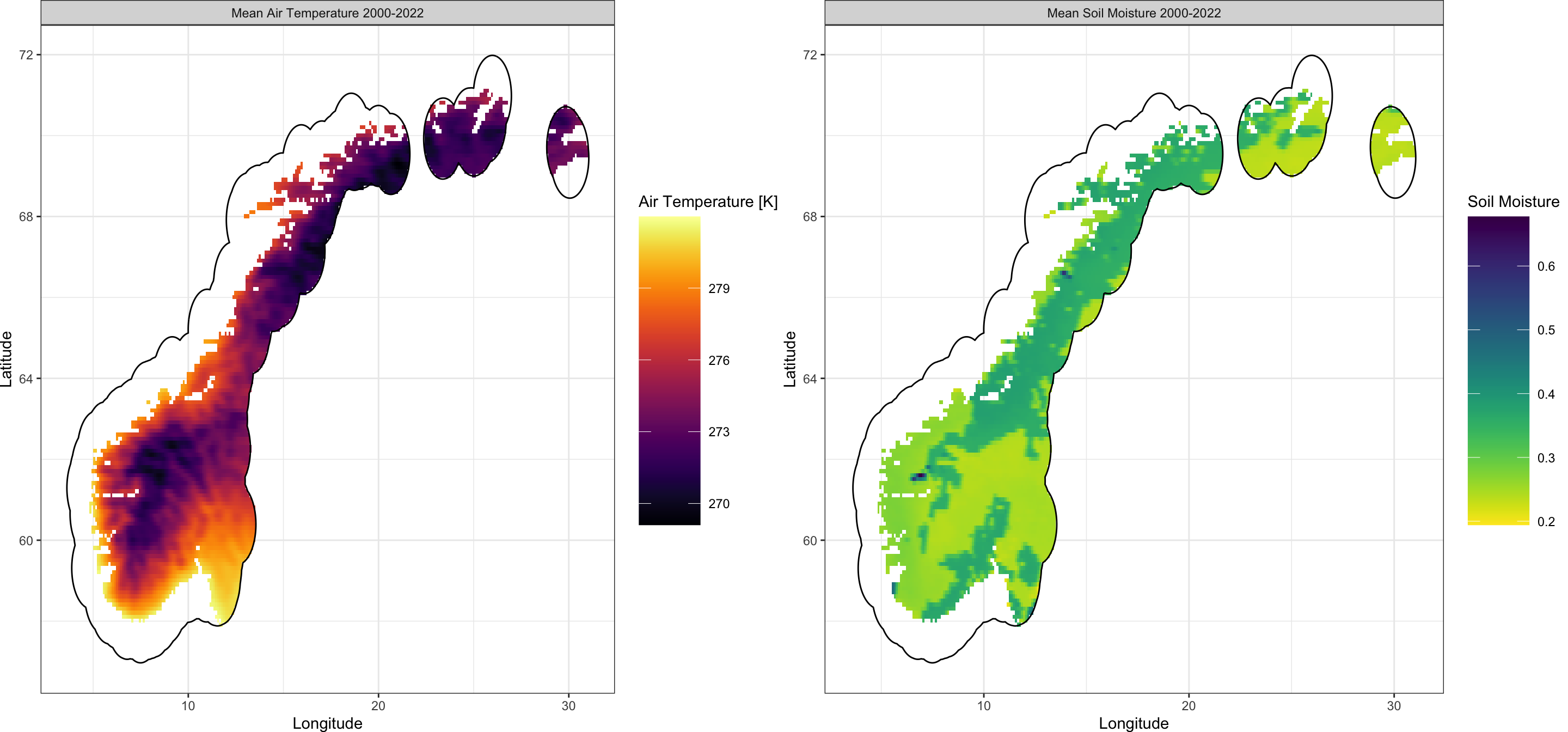
With the above code, we obtain air temperature data as a climatological 23-year mean between 2000 and 2022 for our greater Scandinavian area. We can visualise it as such:
Plot_Raw(AT_ras, Shp = Area_shp, Dates = c("Mean Air Temperature 2000-2022"))

Now let’s do the exact same but for soil moisture data:
QS_ras <- download_ERA(
  Variable = "volumetric_soil_water_layer_1",
  DataSet = "era5-land",
  DateStart = "2000-01-01",
  DateStop = "2022-12-31",
  TResolution = "year",
  TStep = 23,
  Extent = Area_shp,
  Dir = Dir.Data,
  FileName = "QS_ras",
  API_User = API_User,
  API_Key = API_Key,
  SingularDL = TRUE
)
Plot_Raw(QS_ras,
  Shp = Area_shp, COL = rev(viridis(100)),
  Legend = "Soil Moisture",
  Dates = c("Mean Soil Moisture 2000-2022")
)
We now have our two single-layer raster objects corresponding to air temperature and soil moisture ready for matching them to GBIF data.
Bioclimatic Layers
Ultimately, most macroecological uses of GBIF mediated records use some version of bioclimatic variables. Using KrigR, we can obtain these from state-of-the-art climate reanalysis products and even specify more pertinent water variables than the standard precipitation data. Since we are looking at a plant here, probably soil moisture may be most adequate:
if (file.exists(file.path(Dir.Data, "Qsoil_BC.nc"))) {
  BC_ras <- stack(file.path(Dir.Data, "Qsoil_BC.nc"))
  names(BC_ras) <- paste0("BIO", 1:19)
} else {
  BC_ras <- BioClim(
    Water_Var = "volumetric_soil_water_layer_1",
    Y_start = 2000,
    Y_end = 2022,
    Extent = Area_shp,
    Dir = Dir.Data,
    Keep_Monthly = TRUE,
    FileName = "Qsoil_BC.nc",
    API_User = API_User,
    API_Key = API_Key,
    Cores = parallel::detectCores(),
    TimeOut = Inf,
    SingularDL = FALSE
  )
}
The above function call needs to download and process a lot of data hence why I check if the data is already present in the first place. You will see this when running thios function yourself.
Now to visualise the bioclimatic data we have obtained for our study region:
cowplot::plot_grid(
  Plot_BC(BC_ras, Shp = Area_shp, Water_Var = "Soil Moisture", which = 1),
  Plot_BC(BC_ras, Shp = Area_shp, Water_Var = "Soil Moisture", which = 2:19),
  ncol = 1, rel_heights = c(1.3, 9)
)
Matching Climate Data with GBIF Records
To figure out climatological conditions at the locations of our GBIF mediated records, it usually pays to generate a spatial object from our data frame of occurrences:
occ_sp <- data_subset
coordinates(occ_sp) <- ~ decimalLongitude + decimalLatitude
With this, we can now match GBIF records to their local conditions according to our climate data objects.
Single-Layers
Starting with the single-layer rasters, let’s create a stack of them and extract climate values at GBIF presence locations in one step. This creates a wide data frame which, for plotting purposes, we transform into a long format data frame:
SL_stack <- stack(AT_ras, QS_ras)
names(SL_stack) <- c("AT", "QS")
SL_vals <- raster::extract(SL_stack, occ_sp, df = TRUE)
head(SL_vals)
##   ID       AT        QS
## 1  1       NA        NA
## 2  2       NA        NA
## 3  3       NA        NA
## 4  4       NA        NA
## 5  5 278.8715 0.2596406
## 6  6 278.8715 0.2596406
SL_vals <- data.table::melt(na.omit(SL_vals),
  id.vars = "ID"
)
head(SL_vals)
##   ID variable    value
## 1  5       AT 278.8715
## 2  6       AT 278.8715
## 3  7       AT 278.5167
## 4 16       AT 278.5167
## 5 22       AT 278.8715
## 6 25       AT 278.5877
Now, we can plot histograms of climate conditions where we find our study organism:
cols <- list(
  AT = inferno(1e2),
  QS = rev(viridis(1e2))
)
plotlist <- lapply(unique(SL_vals$variable), FUN = function(x) {
  p <- ggplot(SL_vals[SL_vals$variable == x, ], aes(x = value)) +
    geom_histogram(bins = 1e2, fill = cols[[x]]) +
    theme_bw()
  return(p)
})
cowplot::plot_grid(plotlist = plotlist, ncol = 2)
To augment this analysis, we might want to identify climate conditions where our study organism is not found. To not bias this analysis due to our large study region for which we did not query GBIF records, let’s establish a buffer around presence points:
occ_sf <- st_as_sf(occ_sp)
buffer_sf <- st_union(st_buffer(occ_sf, 1)) # 1 degree buffer around points
To visualise this buffer we do the following:
plot(AT_ras)
plot(st_union(buffer_sf), col = "red", add = TRUE)
plot(occ_sf, add = TRUE, col = "black", cex = 0.5, pch = 4)
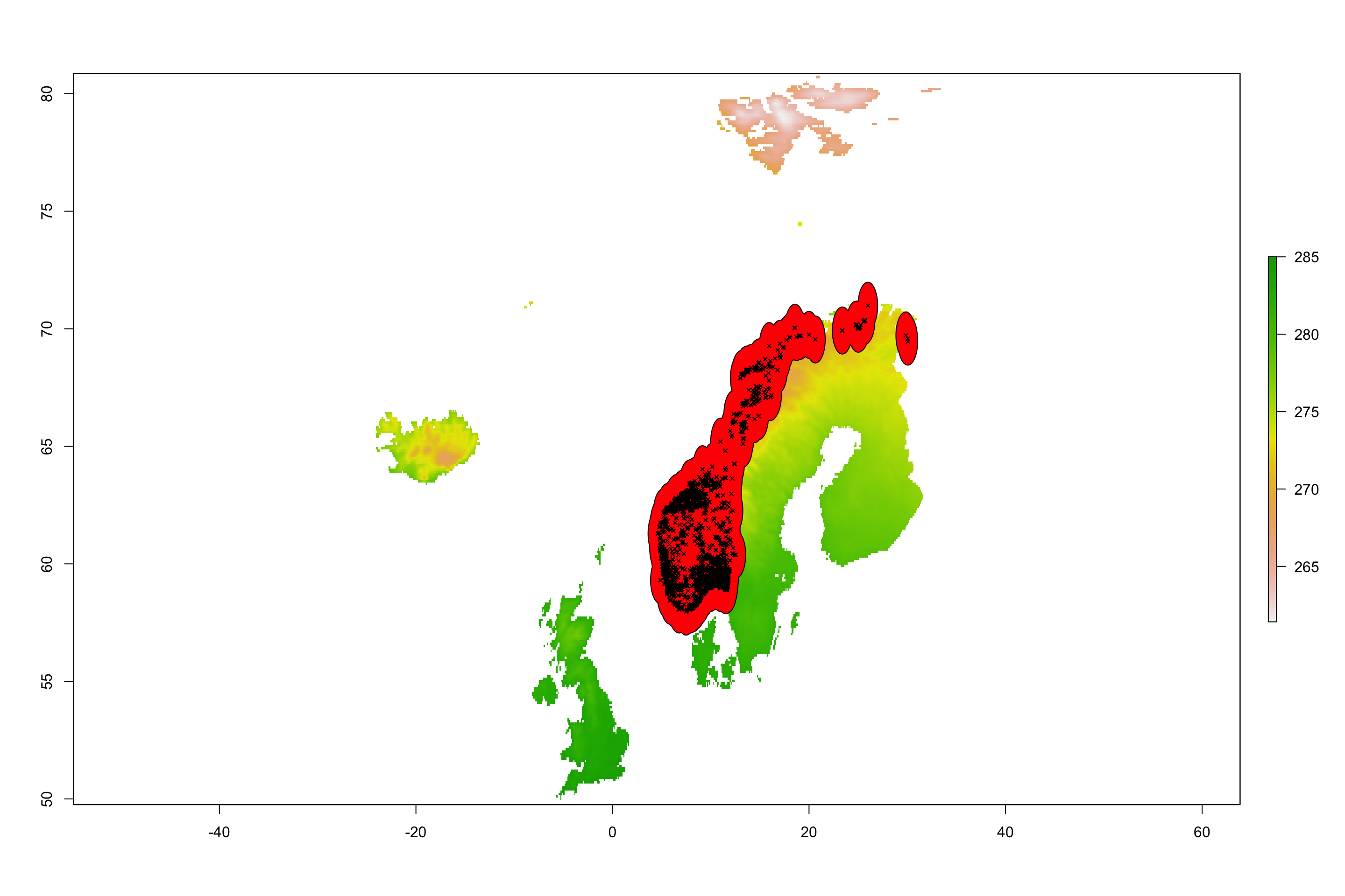
Now we can limit our single-layer climate data to this new buffer area:
SL_crop <- crop(SL_stack, extent(st_bbox(buffer_sf)))
SL_crop <- mask(SL_crop, as(buffer_sf, "Spatial"))
and subsequently visualise the resulting climate data:
cowplot::plot_grid(
  Plot_Raw(SL_crop$AT,
    Shp = as(buffer_sf, "Spatial"),
    Dates = c("Mean Air Temperature 2000-2022")
  ),
  Plot_Raw(SL_crop$QS,
    Shp = as(buffer_sf, "Spatial"),
    COL = rev(viridis(100)),
    Legend = "Soil Moisture",
    Dates = c("Mean Soil Moisture 2000-2022")
  )
)
 Now, we can figure out (1) which cells of this raster contain presences, (2) identify which cells do not, (3) obtain coordinates of cells containing no GBIF presences and (4) extract climate conditions in absence cells:
Pres_cells <- raster::cellFromXY(SL_stack, occ_sp)
Abs_cells <- 1:ncell(SL_stack)[!(1:ncell(SL_stack) %in% Pres_cells)]

SLAbs_vals <- raster::extract(SL_stack,
  raster::xyFromCell(SL_stack, Abs_cells),
  df = TRUE
)
SLAbs_vals <- na.omit(SLAbs_vals)
head(SLAbs_vals)
##        ID       AT         QS
## 1039 1039 266.7161 0.24010955
## 1040 1040 266.7161 0.24010955
## 1041 1041 266.7161 0.24010955
## 1042 1042 266.7161 0.24010955
## 2197 2197 266.4600 0.24119644
## 2778 2778 265.6832 0.09867402
SLAbs_vals <- data.table::melt(SLAbs_vals, id.vars = "ID")
Now to visualise the climate conditions in locations of GBIF presence and absence of our study organism. I also add a t-test comparison between the two presence options to the plot:
SL_vals$Presence <- "Presence"
SLAbs_vals$Presence <- "Absence"
SLPlot_vals <- rbind(SL_vals, SLAbs_vals)
ggplot(SLPlot_vals, aes(
  y = value, x = Presence,
  fill = variable,
  group = Presence
)) +
  geom_violin() +
  geom_boxplot(width = 0.1, fill = "white") +
  stat_compare_means(
    comparisons = list(c("Presence", "Absence")),
    method = "t.test", label = "p.signif"
  ) +
  facet_wrap(~variable, scales = "free") +
  theme_bw() +
  guides(fill = "none")
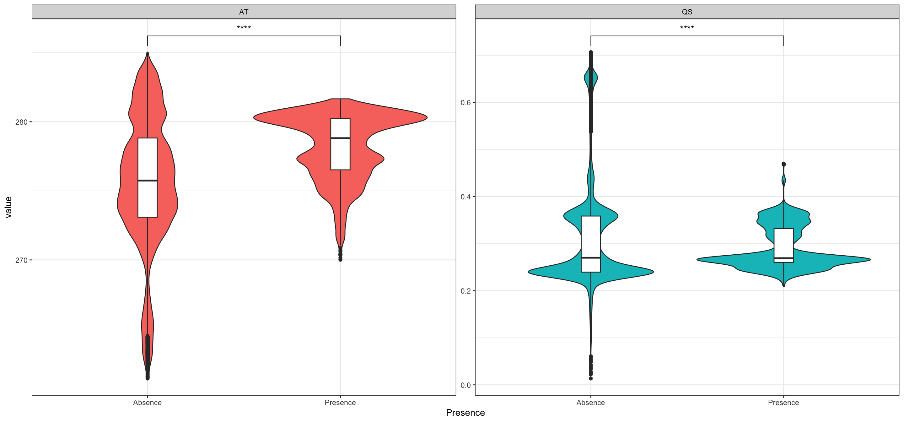
With this in hand, we could now continue to figure out what exactly drives presence and absence of our study organism.
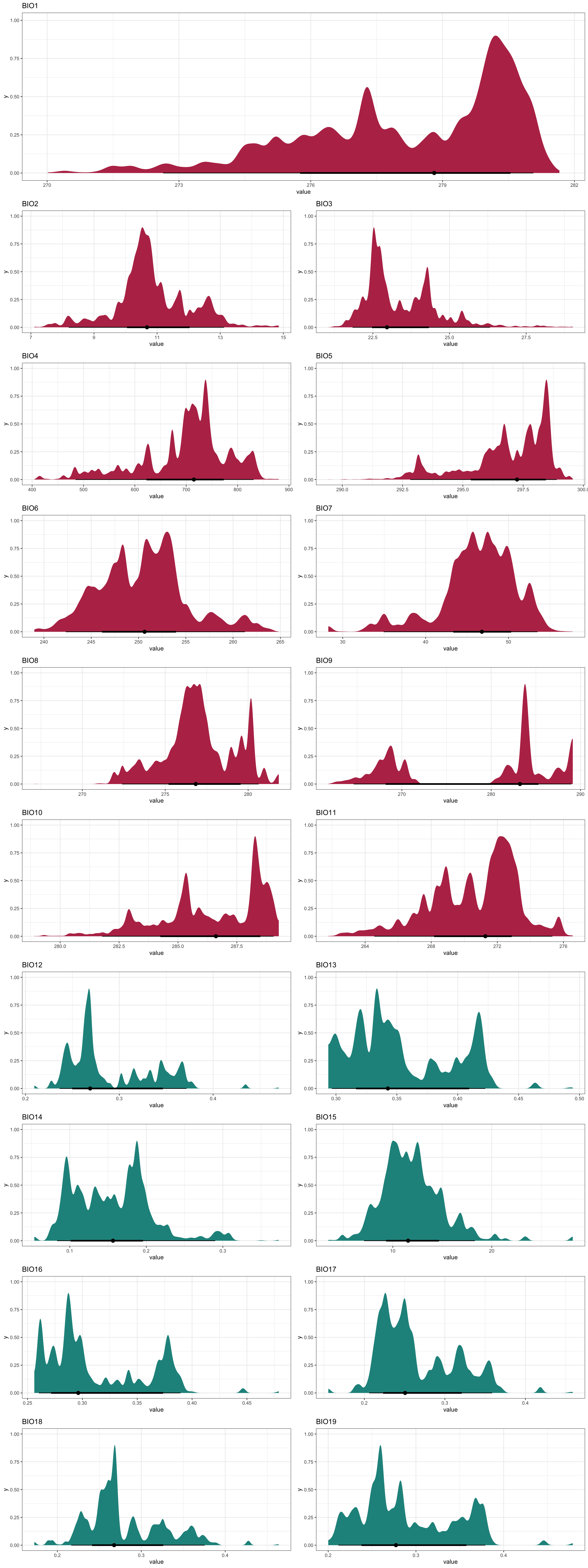
Bioclimatic Variables
Finally, let’s also match our GBIF records with bioclimatic data:
BC_vals <- raster::extract(BC_ras, occ_sp, df = TRUE)
head(BC_vals)
##   ID     BIO1     BIO2     BIO3     BIO4     BIO5     BIO6    BIO7     BIO8     BIO9
## 1  1       NA       NA       NA       NA       NA       NA      NA       NA       NA
## 2  2       NA       NA       NA       NA       NA       NA      NA       NA       NA
## 3  3       NA       NA       NA       NA       NA       NA      NA       NA       NA
## 4  4       NA       NA       NA       NA       NA       NA      NA       NA       NA
## 5  5 278.8715 9.521352 24.52553 531.2745 296.3646 257.5424 38.8222 276.3758 280.5536
## 6  6 278.8715 9.521352 24.52553 531.2745 296.3646 257.5424 38.8222 276.3758 280.5536
##      BIO10    BIO11     BIO12     BIO13     BIO14    BIO15     BIO16     BIO17     BIO18
## 1       NA       NA        NA        NA        NA       NA        NA        NA        NA
## 2       NA       NA        NA        NA        NA       NA        NA        NA        NA
## 3       NA       NA        NA        NA        NA       NA        NA        NA        NA
## 4       NA       NA        NA        NA        NA       NA        NA        NA        NA
## 5 285.4859 273.0706 0.2596402 0.3110663 0.1319089 13.86852 0.2778338 0.2388455 0.2465124
## 6 285.4859 273.0706 0.2596402 0.3110663 0.1319089 13.86852 0.2778338 0.2388455 0.2465124
##       BIO19
## 1        NA
## 2        NA
## 3        NA
## 4        NA
## 5 0.2753689
## 6 0.2753689
BC_vals <- data.table::melt(na.omit(BC_vals), id.vars = "ID")
Again, we create plots for the extracted values. This time however, we use a different frequency visualisation option:
cols <- list(
  AT = inferno(1e2),
  QS = rev(viridis(1e2))
)
plotlist <- lapply(unique(BC_vals$variable), FUN = function(x) {
  y <- ifelse(as.numeric(gsub("\\D", "", x)) < 12, 1, 2)
  p <- ggplot(BC_vals[BC_vals$variable == x, ], aes(x = value)) +
    stat_halfeye(fill = cols[[y]][50]) +
    # geom_histogram(bins = 1e2, fill = cols[[y]]) +
    theme_bw() +
    labs(title = x)
  return(p)
})
cowplot::plot_grid(
  plotlist[[1]],
  cowplot::plot_grid(plotlist = plotlist[-1], ncol = 2),
  ncol = 1, rel_heights = c(1.3, 9)
)
Session Info
## R version 4.3.1 (2023-06-16)
## Platform: x86_64-apple-darwin20 (64-bit)
## Running under: macOS Sonoma 14.1
##
## Matrix products: default
## BLAS:   /Library/Frameworks/R.framework/Versions/4.3-x86_64/Resources/lib/libRblas.0.dylib
## LAPACK: /Library/Frameworks/R.framework/Versions/4.3-x86_64/Resources/lib/libRlapack.dylib;  LAPACK version 3.11.0
##
## locale:
## [1] en_US.UTF-8/en_US.UTF-8/en_US.UTF-8/C/en_US.UTF-8/en_US.UTF-8
##
## time zone: Europe/Oslo
## tzcode source: internal
##
## attached base packages:
## [1] parallel  stats     graphics  grDevices utils     datasets  methods   base
##
## other attached packages:
##  [1] cowplot_1.1.1     viridis_0.6.3     viridisLite_0.4.2 tidyr_1.3.0
##  [5] KrigR_0.1.3       terra_1.7-46      httr_1.4.7        stars_0.6-4
##  [9] abind_1.4-5       fasterize_1.0.4   sf_1.0-14         lubridate_1.9.3
## [13] automap_1.1-9     doSNOW_1.0.20     snow_0.4-4        doParallel_1.0.17
## [17] iterators_1.0.14  foreach_1.5.2     rgdal_1.6-7       raster_3.6-23
## [21] sp_2.0-0          stringr_1.5.0     keyring_1.3.1     ecmwfr_1.5.0
## [25] ncdf4_1.21        ggpubr_0.6.0      data.table_1.14.8 tidybayes_3.0.4
## [29] ggplot2_3.4.3     rgbif_3.7.7
##
## loaded via a namespace (and not attached):
##  [1] tensorA_0.36.2           rstudioapi_0.15.0        jsonlite_1.8.7
##  [4] magrittr_2.0.3           farver_2.1.1             rmarkdown_2.21
##  [7] vctrs_0.6.3              memoise_2.0.1            rstatix_0.7.2
## [10] blogdown_1.16            htmltools_0.5.5          distributional_0.3.2
## [13] curl_5.0.2               broom_1.0.4              sass_0.4.6
## [16] KernSmooth_2.23-21       bslib_0.4.2              plyr_1.8.8
## [19] zoo_1.8-12               cachem_1.0.8             whisker_0.4.1
## [22] lifecycle_1.0.3          pkgconfig_2.0.3          R6_2.5.1
## [25] fastmap_1.1.1            rnaturalearthhires_0.2.1 digest_0.6.31
## [28] colorspace_2.1-0         reshape_0.8.9            labeling_0.4.3
## [31] fansi_1.0.4              urltools_1.7.3           timechange_0.2.0
## [34] compiler_4.3.1           proxy_0.4-27             intervals_0.15.4
## [37] bit64_4.0.5              withr_2.5.1              backports_1.4.1
## [40] carData_3.0-5            DBI_1.1.3                highr_0.10
## [43] R.utils_2.12.2           ggsignif_0.6.4           classInt_0.4-10
## [46] oai_0.4.0                tools_4.3.1              units_0.8-4
## [49] R.oo_1.25.0              glue_1.6.2               R.cache_0.16.0
## [52] grid_4.3.1               checkmate_2.2.0          reshape2_1.4.4
## [55] generics_0.1.3           gtable_0.3.4             R.methodsS3_1.8.2
## [58] class_7.3-22             xml2_1.3.4               car_3.1-2
## [61] utf8_1.2.3               pillar_1.9.0             ggdist_3.3.0
## [64] posterior_1.4.1          dplyr_1.1.2              lattice_0.21-8
## [67] FNN_1.1.3.2              bit_4.0.5                tidyselect_1.2.0
## [70] knitr_1.43               arrayhelpers_1.1-0       gridExtra_2.3
## [73] bookdown_0.34            crul_1.4.0               xfun_0.39
## [76] stringi_1.7.12           lazyeval_0.2.2           yaml_2.3.7
## [79] evaluate_0.20            codetools_0.2-19         httpcode_0.3.0
## [82] tibble_3.2.1             cli_3.6.1                munsell_0.5.0
## [85] jquerylib_0.1.4          styler_1.9.1             spacetime_1.3-0
## [88] Rcpp_1.0.11              rnaturalearth_0.3.2      triebeard_0.4.1
## [91] coda_0.19-4              svUnit_1.0.6             assertthat_0.2.1
## [94] scales_1.2.1             xts_0.13.1               e1071_1.7-13
## [97] gstat_2.1-1              purrr_1.0.1              rlang_1.1.1