Handling Data with rgbif

## Custom install & load function
install.load.package <- function(x) {
  if (!require(x, character.only = TRUE)) {
    install.packages(x, repos = "http://cran.us.r-project.org")
  }
  require(x, character.only = TRUE)
}
## names of packages we want installed (if not installed yet) and loaded
package_vec <- c(
  "rgbif",
  "knitr", # for rmarkdown table visualisations
  "sp", # for spatialobject creation
  "sf", # an alternative spatial object library
  "ggplot2", # for visualistion
  "maptools", # for visualisation
  "rgeos", # for visualisation
  "raster", # for setting and reading CRS
  "rnaturalearth" # for shapefiles of naturalearth
)
## executing install & load for each package
sapply(package_vec, install.load.package)

##         rgbif         knitr            sp            sf       ggplot2      maptools 
##          TRUE          TRUE          TRUE          TRUE          TRUE          TRUE 
##         rgeos        raster rnaturalearth 
##          TRUE          TRUE          TRUE

options(gbif_user = "my gbif username")
options(gbif_email = "my registred gbif e-mail")
options(gbif_pwd = "my gbif password")

First, we obtain and load the data we are interested in like such:

# Download query
res <- occ_download(
  pred("taxonKey", sp_key),
  pred_in("basisOfRecord", c("HUMAN_OBSERVATION")),
  pred("country", "NO"),
  pred("hasCoordinate", TRUE),
  pred_gte("year", 2000),
  pred_lte("year", 2022)
)
# Downloading and Loading
res_meta <- occ_download_wait(res, status_ping = 5, curlopts = list(), quiet = FALSE)
res_get <- occ_download_get(res)
res_data <- occ_download_import(res_get)

With this data in our R environment, we are ready to explore the data itself.

Initial Data Handling

Before working with the data you obtained via GBIF, it is usually good practice to first check that all data is as expected/in order and then either reduce the dataset further to fit quality standards and extract the relevant variables for your application.

Common Data Considerations & Issues

Common data considerations and quality flags are largely related to geolocations (but other quality markers do exist). These can be used as limiting factors in data discovery, when querying downloads as well as after a download is done and the data is loaded. Within the GBIF Portal, these options are presented in a side-bar like this:

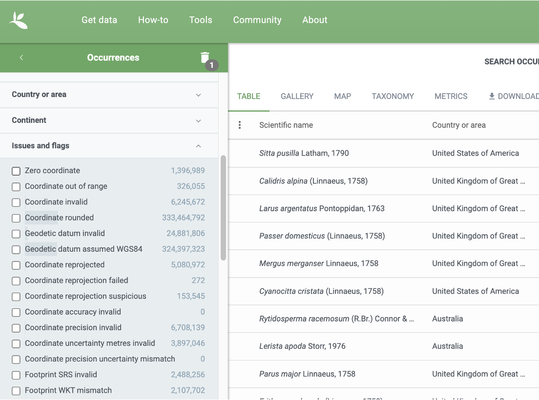
As a matter of fact, we have already used the functionality by which to control for data quality markers when carrying out data discovery (occ_search(...)) and data download queries (occ_download(...)) by matching Darwin Core Terms like basisOfRecord or hasCoordinate.

For this exercise, let’s focus on some data markers that are contained in our already downloaded data set which we may want to use for further limiting of our data set for subsequent analyses. To do so, let’s consider the coordinateUncertaintyInMeters field by visualising the values we have obtained for each record in our occurrence data:

ggplot(res_data, aes(x = coordinateUncertaintyInMeters)) +
  geom_histogram(bins = 1e2) +
  theme_bw() +
  scale_y_continuous(trans = "log10")

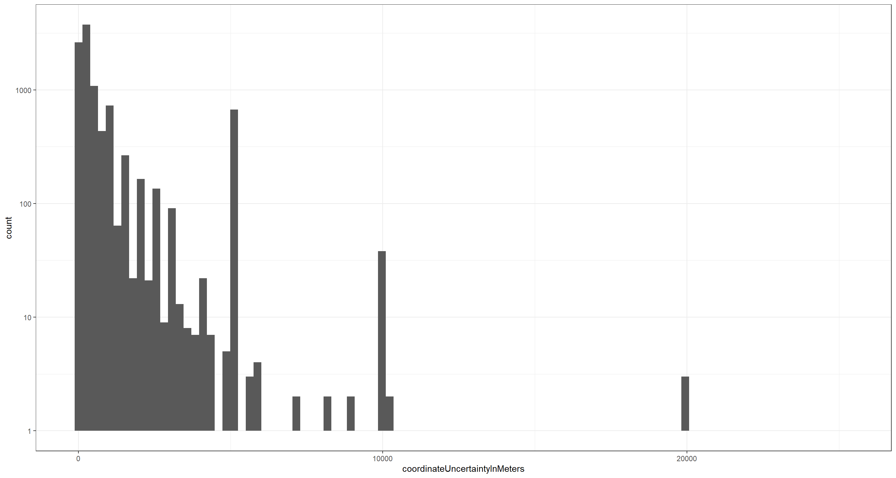
Note: The y-axis on the above plot is log-transformed and 1053 of the underlying records do not report a value for coordinateUncertaintyInMeters thus being removed from the above visualisation.

What we find is that there exists considerable variation in confidence of individual occurrence locations and we probably want to remove those records which are assigned a certain level of coordinateUncertaintyInMeters. Let’s say 10 metres:

preci_data <- res_data[which(res_data$coordinateUncertaintyInMeters < 10), ]

This quality control leaves us with 6802 Calluna vulgaris records. A significant drop in data points which may well change our analyses and their outcomes drastically.

Extract a Subset of Cata-Columns

GBIF mediated data comes with a lot of attributes. These can be assessed readily via the Darwin Core or, within R via: colnames(...) (here with ... = res_data). Rarely will we need all of them for our analyses. For now, we will simply subset the data for a smaller set of columns which are often relevant for end-users:

data_subset <- preci_data[
  ,
  c("scientificName", "decimalLongitude", "decimalLatitude", "basisOfRecord", "year", "month", "day", "eventDate", "countryCode", "municipality", "taxonKey", "species", "catalogNumber", "hasGeospatialIssues", "hasCoordinate", "datasetKey")
]
knitr::kable(head(data_subset))

Explore the Occurrence Data

Now that we have the data we might use for analyses ready, we can explore what the data itself contains.

Data Contents

Here are a few overviews of Calluna vulgaris abundances across different data attributes:

table(data_subset$year)

## 
## 2000 2001 2002 2003 2004 2005 2006 2007 2008 2009 2010 2011 2012 2013 2014 2015 2016 2017 
##    2    5    1   11    4    8    8   12   37  313  509  380  255  255  349  404  505  502 
## 2018 2019 2020 2021 2022 
##  256  369  427 1022 1168

table(data_subset$stateProvince)

## < table of extent 0 >

table(data_subset$mediaType)

## < table of extent 0 >

Spatial Data Handling

Most use-cases of GBIF make use of the geolocation references for data records either implicitly or explicitly. It is thus vital to be able to handle GBIF mediated data for spatial analyses. There exist plenty workshop (like this one) already for this topic so I will be brief.

Make SpatialPointsDataFrame

First, we can use the sp package to create SpatialPoints from our geo-referenced occurrence data:

options(digits = 8) ## set 8 digits (ie. all digits, not decimals) for the type cast as.double to keep decimals
data_subset <- as.data.frame(data_subset)
data_subset$lon <- as.double(data_subset$decimalLongitude) ## cast lon from char to double
data_subset$lat <- as.double(data_subset$decimalLatitude) ## cast lat from char to double
coordinates(data_subset) <- ~ lon + lat ## make data_subset into SpatialPointsDataFrame
proj4string(data_subset) <- CRS("+proj=longlat +ellps=WGS84 +datum=WGS84 +no_defs +towgs84=0,0,0") ## set CRS

This data format lends itself well for analysing where occurrence have been recorded in relation to study parameters of choice (e.g., climatic conditions, land-use, political boundaries, etc.).

SpatialPoints and Polygons

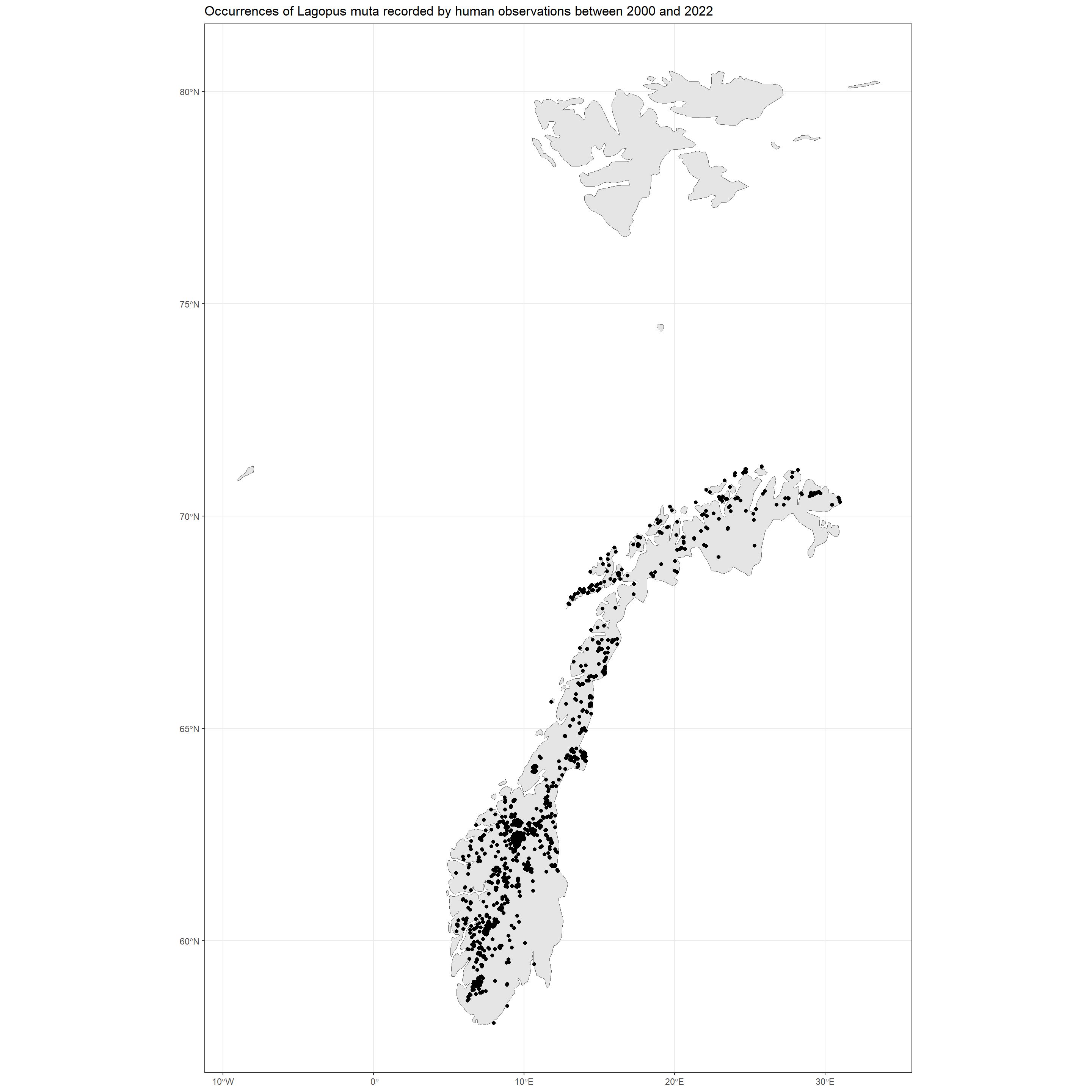
In first instance, SpatialPoints can easily be used to create initial visualisations of spatial patterns:

## Data Handling
data_xy <- data_subset[c("decimalLongitude", "decimalLatitude")] ## Extract only the coordinates
data(wrld_simpl)
norway_mask <- subset(wrld_simpl, NAME == "Norway")
## Plotting
plot(norway_mask, axes = TRUE)
title("Calluna vulgaris presences recorded by human observation between 2000 and 2022 across Norway")
points(data_xy, col = "red", pch = 20, cex = 1) # plot species occurrence points to the map
legend("bottomright", title = "Legend", legend = "Occurrences", pch = 20, col = "red", cex = 0.9)

The Coordinate Reference System (CRS)

Each spatial object in R is assigned a Coordinate Reference System (CRS) which details how geolocational values are to be understood. For an overview of different CRSs, see here.

In R, we can assess the CRS of most spatial objects as follows:

raster::crs(wrld_simpl)

## Coordinate Reference System:
## Deprecated Proj.4 representation:
##  +proj=longlat +ellps=WGS84 +towgs84=0,0,0,0,0,0,0 +no_defs 
## WKT2 2019 representation:
## GEOGCRS["unknown",
##     DATUM["World Geodetic System 1984",
##         ELLIPSOID["WGS 84",6378137,298.257223563,
##             LENGTHUNIT["metre",1]],
##         ID["EPSG",6326]],
##     PRIMEM["Greenwich",0,
##         ANGLEUNIT["degree",0.0174532925199433],
##         ID["EPSG",8901]],
##     CS[ellipsoidal,2],
##         AXIS["longitude",east,
##             ORDER[1],
##             ANGLEUNIT["degree",0.0174532925199433,
##                 ID["EPSG",9122]]],
##         AXIS["latitude",north,
##             ORDER[2],
##             ANGLEUNIT["degree",0.0174532925199433,
##                 ID["EPSG",9122]]]]

raster::crs(data_subset)

## Coordinate Reference System:
## Deprecated Proj.4 representation: +proj=longlat +datum=WGS84 +no_defs 
## WKT2 2019 representation:
## GEOGCRS["unknown",
##     DATUM["World Geodetic System 1984",
##         ELLIPSOID["WGS 84",6378137,298.257223563,
##             LENGTHUNIT["metre",1]],
##         ID["EPSG",6326]],
##     PRIMEM["Greenwich",0,
##         ANGLEUNIT["degree",0.0174532925199433],
##         ID["EPSG",8901]],
##     CS[ellipsoidal,2],
##         AXIS["longitude",east,
##             ORDER[1],
##             ANGLEUNIT["degree",0.0174532925199433,
##                 ID["EPSG",9122]]],
##         AXIS["latitude",north,
##             ORDER[2],
##             ANGLEUNIT["degree",0.0174532925199433,
##                 ID["EPSG",9122]]]]

When dealing with data in specific areas of the world or wanting to match occurrence data to other products with specific CRSs, it may be prudent to reproject the SpatialPoints occurrence data object. We can use sp:spTransform() to do so (this is reprojecting to the same CRS the data is already in):

sp::spTransform(data_subset, CRS("+proj=longlat +ellps=WGS84 +datum=WGS84 +no_defs +towgs84=0,0,0"))

## class       : SpatialPointsDataFrame 
## features    : 6802 
## extent      : 4.619497, 30.051781, 57.969404, 70.981838  (xmin, xmax, ymin, ymax)
## crs         : +proj=longlat +datum=WGS84 +no_defs 
## variables   : 16
## names       :             scientificName, decimalLongitude, decimalLatitude,     basisOfRecord, year, month, day,  eventDate, countryCode, municipality, taxonKey,          species, catalogNumber, hasGeospatialIssues, hasCoordinate, ... 
## min values  : Calluna vulgaris (L.) Hull,         4.619497,       57.969404, HUMAN_OBSERVATION, 2000,     1,   1,  961891200,          NO,             ,  2882482, Calluna vulgaris,              ,                   0,             1, ... 
## max values  : Calluna vulgaris (L.) Hull,        30.051781,       70.981838, HUMAN_OBSERVATION, 2022,    12,  31, 1671235200,          NO,         Voss,  2882482, Calluna vulgaris, OBS.259608743,                   0,             1, ...

Classifying Spatial Data

Moving from the relatively limited sp package to the more functional sf package enables more advanced visualisations of additional spatial considerations of our data.

For example, consider we want to quantify abundances of Calluna vulgaris across political regions in Norway:

## Obtain sf object
data_sf <- st_as_sf(data_subset) # make sp into sf
NO_municip <- rnaturalearth::ne_states(country = "Norway", returnclass = "sf") # get shapefiles for Norwegian states
NO_municip <- sf::st_crop(NO_municip, extent(4.5, 31.5, 50, 71.5)) # crop shapefile to continental Norway
## Identify overlap of points and polygons
cover_sf <- st_intersects(NO_municip, data_sf)
names(cover_sf) <- NO_municip$name
## report abundances
abundances_municip <- unlist(lapply(cover_sf, length))
sort(abundances_municip, decreasing = TRUE)

##          Østfold  Møre og Romsdal         Buskerud       Vest-Agder         Telemark 
##             1838             1173              366              315              283 
##         Rogaland         Akershus        Hordaland       Aust-Agder    Sør-Trøndelag 
##              263              199              197              172              150 
##         Nordland          Hedmark Sogn og Fjordane             Oslo          Oppland 
##              129              127              115              106              104 
##         Vestfold   Nord-Trøndelag         Finnmark            Troms 
##               82               31               28               12

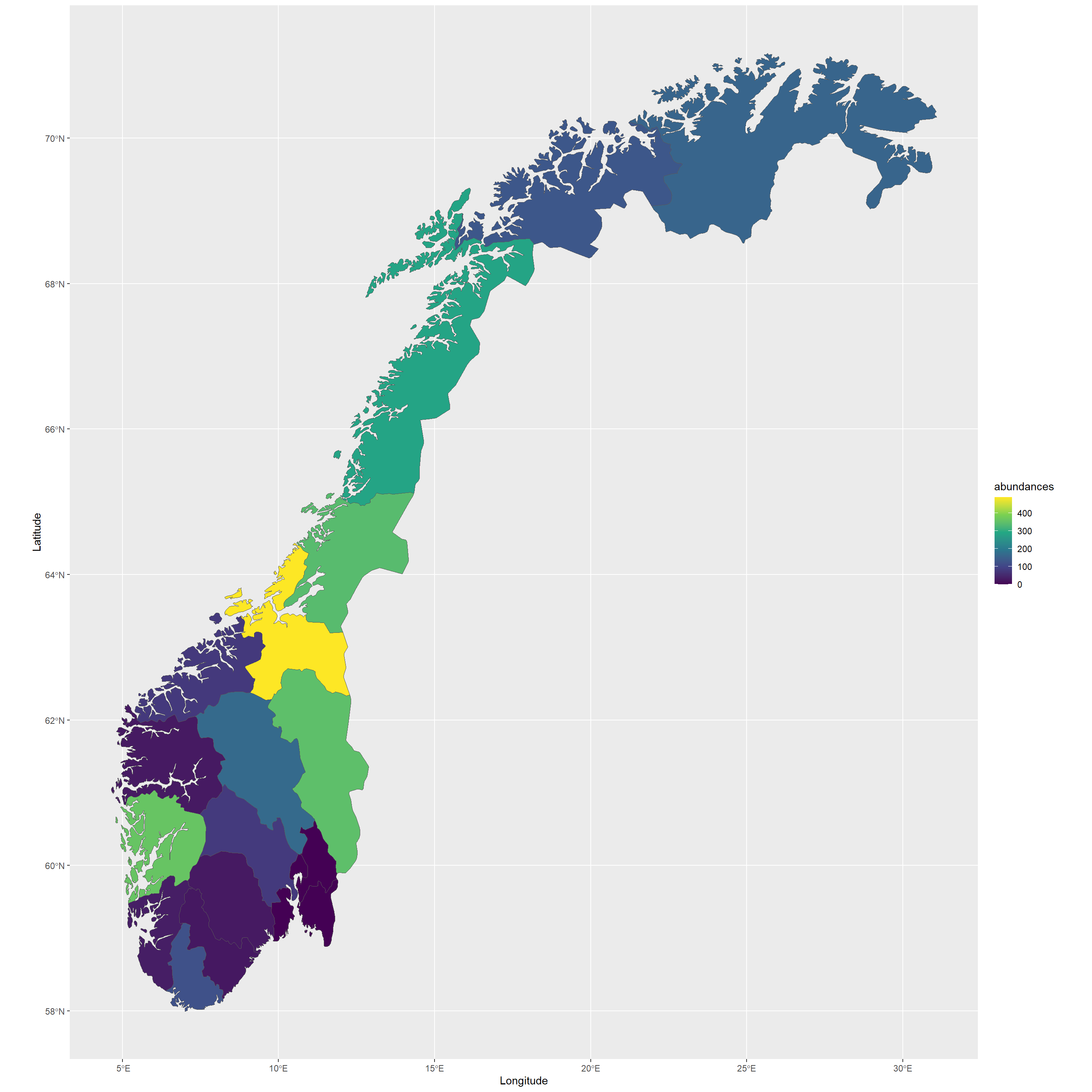
Looks like there are hotspots for Calluna vulgaris in Østfold and Møre og Romsdal - could this be sampling bias or effects of bioclimatic niche preferences and local environmental conditions? Questions like these you will be able to answer with additional analyses which are beyond the scope of this workshop.

Let’s visualise these abundances:

NO_municip$abundances <- abundances_municip
ggplot(data = NO_municip) +
  geom_sf(aes(fill = abundances)) +
  scale_fill_viridis_c() +
  labs(x = "Longitude", y = "Latitude", col = "Abundance")

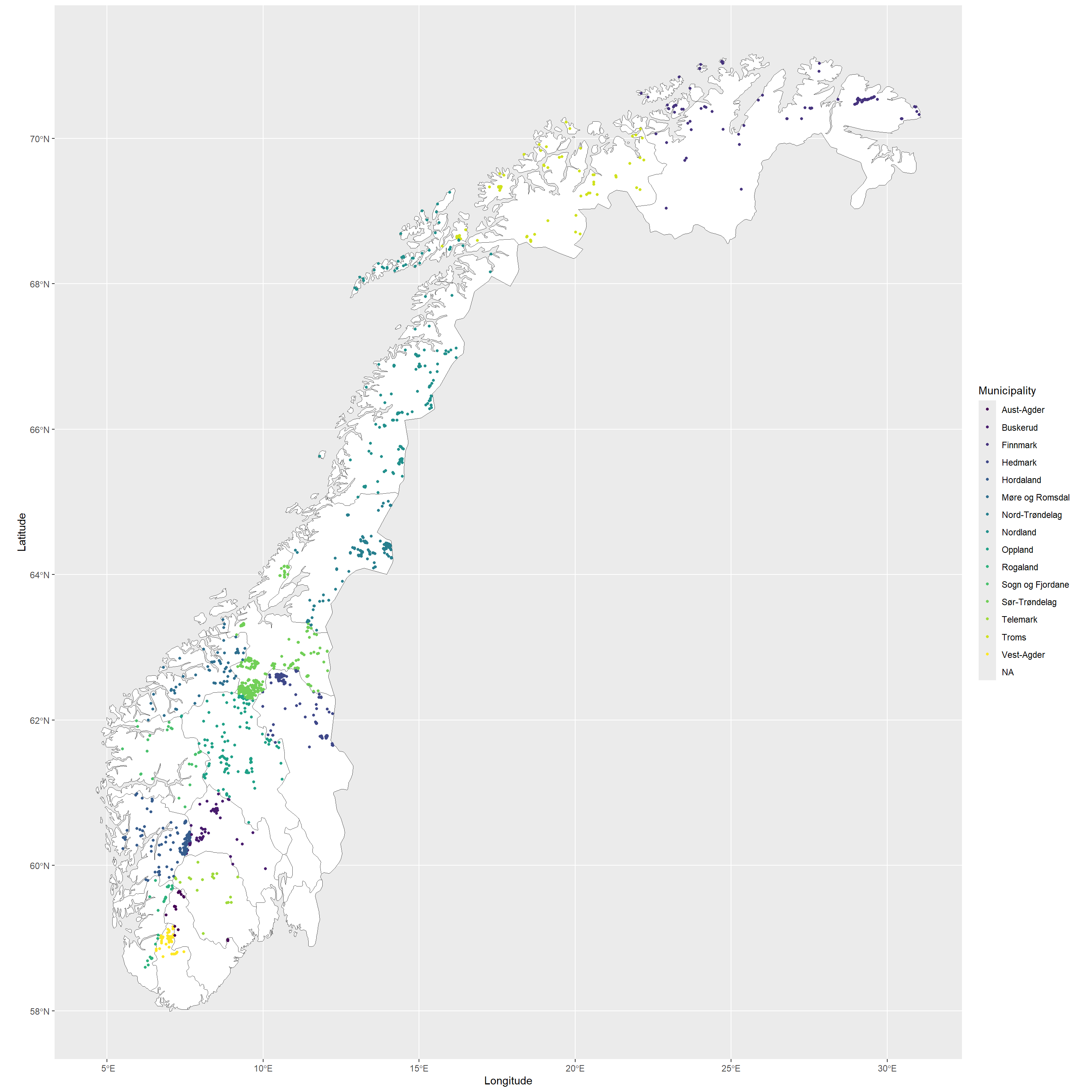
Finally, let’s consider wanting to identify for each data record and attach to the data itself which state it falls into. We can do so as follows (not necessarily the most elegant way:

## create a dataframe of occurrence records by rownumber in original data (data_subset) and state-membership
cover_ls <- lapply(names(cover_sf), FUN = function(x) {
  data.frame(
    municip = x,
    points = cover_sf[[x]]
  )
})
cover_df <- do.call(rbind, cover_ls)
## attach state-membership to original data, NAs for points without state-membership
data_subset$municip <- NA
data_subset$municip[cover_df$points] <- cover_df$municip
## visualise the result
ggplot(data = NO_municip) +
  geom_sf(fill = "white") +
  geom_point(
    data = data_subset@data, size = 1,
    aes(x = decimalLongitude, y = decimalLatitude, col = municip)
  ) +
  scale_colour_viridis_d() +
  labs(x = "Longitude", y = "Latitude", col = "Municipality")

Let’s say we feed these data into an analysis which runs to completion and we want to report on our findings. What’s next? Citing the data we used.

Session Info

## R version 4.3.0 (2023-04-21)
## Platform: x86_64-apple-darwin20 (64-bit)
## Running under: macOS Ventura 13.3.1
## 
## Matrix products: default
## BLAS:   /Library/Frameworks/R.framework/Versions/4.3-x86_64/Resources/lib/libRblas.0.dylib 
## LAPACK: /Library/Frameworks/R.framework/Versions/4.3-x86_64/Resources/lib/libRlapack.dylib;  LAPACK version 3.11.0
## 
## locale:
## [1] en_US.UTF-8/en_US.UTF-8/en_US.UTF-8/C/en_US.UTF-8/en_US.UTF-8
## 
## time zone: Europe/Oslo
## tzcode source: internal
## 
## attached base packages:
## [1] stats     graphics  grDevices utils     datasets  methods   base     
## 
## other attached packages:
## [1] rnaturalearth_0.3.2 raster_3.6-20       rgeos_0.6-2         maptools_1.1-6     
## [5] ggplot2_3.4.2       sf_1.0-12           sp_1.6-0            knitr_1.42         
## [9] rgbif_3.7.7        
## 
## loaded via a namespace (and not attached):
##  [1] gtable_0.3.3             xfun_0.39                bslib_0.4.2             
##  [4] lattice_0.21-8           vctrs_0.6.2              tools_4.3.0             
##  [7] generics_0.1.3           curl_5.0.0               tibble_3.2.1            
## [10] proxy_0.4-27             fansi_1.0.4              highr_0.10              
## [13] pkgconfig_2.0.3          R.oo_1.25.0              KernSmooth_2.23-20      
## [16] data.table_1.14.8        lifecycle_1.0.3          R.cache_0.16.0          
## [19] farver_2.1.1             compiler_4.3.0           stringr_1.5.0           
## [22] munsell_0.5.0            terra_1.7-29             codetools_0.2-19        
## [25] htmltools_0.5.5          class_7.3-21             sass_0.4.6              
## [28] yaml_2.3.7               lazyeval_0.2.2           pillar_1.9.0            
## [31] jquerylib_0.1.4          whisker_0.4.1            R.utils_2.12.2          
## [34] classInt_0.4-9           cachem_1.0.8             wk_0.7.2                
## [37] styler_1.9.1             tidyselect_1.2.0         digest_0.6.31           
## [40] stringi_1.7.12           dplyr_1.1.2              purrr_1.0.1             
## [43] bookdown_0.34            labeling_0.4.2           fastmap_1.1.1           
## [46] grid_4.3.0               colorspace_2.1-0         cli_3.6.1               
## [49] magrittr_2.0.3           triebeard_0.4.1          crul_1.4.0              
## [52] utf8_1.2.3               e1071_1.7-13             foreign_0.8-84          
## [55] withr_2.5.0              scales_1.2.1             bit64_4.0.5             
## [58] oai_0.4.0                rmarkdown_2.21           httr_1.4.5              
## [61] bit_4.0.5                blogdown_1.16            rnaturalearthhires_0.2.1
## [64] R.methodsS3_1.8.2        evaluate_0.20            rgdal_1.6-6             
## [67] viridisLite_0.4.2        s2_1.1.3                 urltools_1.7.3          
## [70] rlang_1.1.1              Rcpp_1.0.10              httpcode_0.3.0          
## [73] glue_1.6.2               DBI_1.1.3                xml2_1.3.4              
## [76] rstudioapi_0.14          jsonlite_1.8.4           R6_2.5.1                
## [79] plyr_1.8.8               units_0.8-2