Chapter 12
Monsters & Mixtures
Material
Introduction
These are answers and solutions to the exercises at the end of chapter 12 in Satistical Rethinking 2 by Richard McElreath. I have created these notes as a part of my ongoing involvement in the AU Bayes Study Group. Much of my inspiration for these solutions, where necessary, has been obtained from
the solutions provided to instructors by Richard McElreath himself.
R Environment
For today’s exercise, I load the following packages:
library(rethinking)
library(rstan)
library(ggplot2)
library(tidybayes)
Easy Exercises
Practice E1
Question: What is the difference between an ordered categorical variable and an unordered one? Define and then give an example of each.
Answer:
Ordered categorical variables are those which are expressed on ordinal scales. Not very helpful, right? Well, these are variables which establish a pre-defined number of distinct outcomes. These may be expressed as numbers, but don’t have to be. What’s special about these variables is that their values (i.e. categories) can be ordered meaningfully from one extreme to the another without implying equal distances between the values. As an example, think of sparrow (Passer domesticus) weight. We may have measured these in grams (as a continuous variable), but now want to model simply whether our sparrows are light-, medium-, or heavy-weights. This is an ordered categorical variable because we now how they can be ordered from one extreme to another, but we don’t assume that a sparrow has to become heavier by the same margin to classify as medium-weight instead of light-weight than to classify as heavy-weight instead of medium-weight.
Unordered categorical variables are much like their ordered counterpart, but come with an important distinction: we cannot order these in any meaningful way. Again, think of the common house sparrow (Passer domesticus) and their colouration patterns. We may want to record them as overall black, brown, or grey. These are categories, but we certainly cannot order these from one extreme to another.
Practice E2
Question: What kind of link function does an ordered logistic regression employ? How does it differ from an ordinary logit link?
Answer:
Cumulative logit - $OrdLogit( = \phi, K)$. This link function defines a number of $K-1$ cumulative, proportional probabilities ($\phi$) of each outcome category. The $K-1$ $\phi_i$ sum up to 1 so that the $\phi_K = 1$ and can subsequently be dropped from the model. The link thus states that the linear model defines the log-cumulative odds of an event.
Practice E3
Question: When count data are zero-inflated, using a model that ignores zero-inflation will tend to induce which kind of inferential error?
Answer:
Under-prediction of the true rate of events. Zero-inflation means that counts of zero arise through more than one process at least one of which is not accounted for in our model. Subsequently our estimate of the true rate will be pushed closer to 0 than it truly is.
Practice E4
Question: Over-dispersion is common in count data. Give an example of a natural process that might produce over-dispersed counts. Can you also give an example of a process that might produce under- dispersed counts?
Answer:
Over-dispersion often comes about as a result of heterogeneity in rates across different sampling units/systems. As an example, think of lizard counts in different patches of a dryland area over a given period of time. The resulting count data will likely be over-dispersed since the rate at which lizards are observed will vary strongly across the different study sites.
Under-dispersion, on the other hand, shows less variation in the rates than would be expected. This is often the case when autocrrelation plays a role. For example, if we track our lizard abundances at each patch through time in half-day intervals, we are likely to end up with highly autocorrelated and under-dispersed counts/rates for each study site.
Medium Exercises
Practice M1
Question: At a certain university, employees are annually rated from 1 to 4 on their productivity, with 1 being least productive and 4 most productive. In a certain department at this certain university in a certain year, the numbers of employees receiving each rating were (from 1 to 4): 12, 36, 7, 41. Compute the log cumulative odds of each rating.
Answer:
n <- c(12, 36, 7, 41) # assignment
q <- n / sum(n) # proportions
p <- cumsum(q) # cumulative proportions
o <- p / (1 - p) # cumulative odds
log(o) # log-cumulative odds
## [1] -1.9459101 0.0000000 0.2937611 Inf
Practice M2
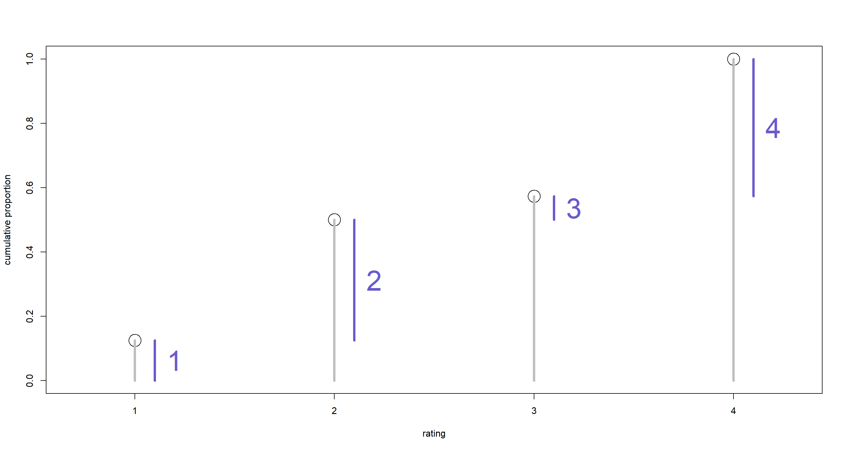
Question: Make a version of Figure 12.5 for the employee ratings data given just above.
Answer:
# plot raw proportions
plot(1:4, p,
  xlab = "rating", ylab = "cumulative proportion",
  xlim = c(0.7, 4.3), ylim = c(0, 1), xaxt = "n", cex = 3
)
axis(1, at = 1:4, labels = 1:4)
# plot gray cumulative probability lines
for (x in 1:4) lines(c(x, x), c(0, p[x]), col = "gray", lwd = 4)
# plot blue discrete probability segments
for (x in 1:4) lines(c(x, x) + 0.1, c(p[x] - q[x], p[x]), col = "slateblue", lwd = 4)
# add number labels
text(1:4 + 0.2, p - q / 2, labels = 1:4, col = "slateblue", cex = 3)
Practice M3
Question: Can you modify the derivation of the zero-inflated Poisson distribution (ZIPoisson) from the chapter to construct a zero-inflated binomial distribution?
Answer:
Let’s remind ourselves of the ZI-Poisson distribution from the chapter:
$$ ZIPoisson(p, \lambda) $$
with:
- p = probability of no count generating process occurring
- λ = rate at which counts are produced when process occurs
This is an extension of the Poisson distribution which is in itself a special version of the Binomial distribution with many trials and a low success rate. The zero-inflated Poisson may also be expressed as ($F$ and $S$ indicate binomial process has succeeded or failed in prohibiting the poisson process from happening, respectively):
$$Pr(0|p_0, λ) = Pr(F|p_0) + Pr(S|p_0)*Pr(0|λ) = p_0 + (1 − p_0) * exp(−λ)$$ For zero-observations.
$$Pr(y|y>0,p_0,\lambda) = Pr(S|p_0)(0) + Pr(F|p_0)*Pr(y|\lambda) = (1-p_0)\frac{\lambda^yexp(-\lambda)}{y!}$$ For non zero-observations.
So how do we now get to a binomial specification here? By changing the Poisson likelihood ($exp(−λ)$) to a Binomial likelihood ($(1 − q)^n$ with $q$ denoting the probability of success):
$$Pr(0|p_0, q, n) = p_0 + (1 − p_0)(1 − q)^n$$ For zero-observations.
$$Pr(y|p_0, q, n) = (1 − p_0) Binom(y, n, q) = (1 − p_0) \frac{n!}{y!(n − y)!}*q^y(1 − q)^{n−y}$$ For non zero-observations.
Hard Exercises
Practice H1
Question: In 2014, a paper was published that was entitled “Female hurricanes are deadlier than male hurricanes.” As the title suggests, the paper claimed that hurricanes with female names have caused greater loss of life, and the explanation given is that people unconsciously rate female hurricanes as less dangerous and so are less likely to evacuate. Statisticians severely criticized the paper after publication. Here, you’ll explore the complete data used in the paper and consider the hypothesis that hurricanes with female names are deadlier. Load the data with:
library(rethinking)
data(Hurricanes)
Acquaint yourself with the columns by inspecting the help ?Hurricanes. In this problem, you’ll focus on predicting deaths using femininity of each hurricane’s name.
Fit and interpret the simplest possible model, a Poisson model of deaths using femininity as a predictor. You can use quap or ulam. Compare the model to an intercept-only Poisson model of deaths. How strong is the association between femininity of name and deaths? Which storms does the model fit (retrodict) well? Which storms does it fit poorly?
Answer: First, let’s prepare the data:
d <- Hurricanes # load data on object called d
d$fem_std <- (d$femininity - mean(d$femininity)) / sd(d$femininity) # standardised femininity
dat <- list(D = d$deaths, F = d$fem_std)
Now that we have standardised data for the feminity of our hurricane names which makes priors easier to formulate, we can specify our initial model idea:
# model formula
f <- alist(
  D ~ dpois(lambda), # poisson outcome distribution
  log(lambda) <- a + bF * F, # log-link for lambda with linear model
  # priors in log-space, 0 corresponds to outcome of 1
  a ~ dnorm(1, 1),
  bF ~ dnorm(0, 1)
)
But are these priors any good? Let’s simulate them why don’t we:
N <- 1e3
a <- rnorm(N, 1, 1)
bF <- rnorm(N, 0, 1)
F_seq <- seq(from = -2, to = 2, length.out = 30) # sequence from -2 to 2 because femininity data is standardised
plot(NULL,
  xlim = c(-2, 2), ylim = c(0, 500),
  xlab = "name femininity (std)", ylab = "deaths"
)
for (i in 1:N) {
  lines(F_seq,
    exp(a[i] + bF[i] * F_seq), # inverse link to get outcome scale
    col = grau(), lwd = 1.5
  )
}
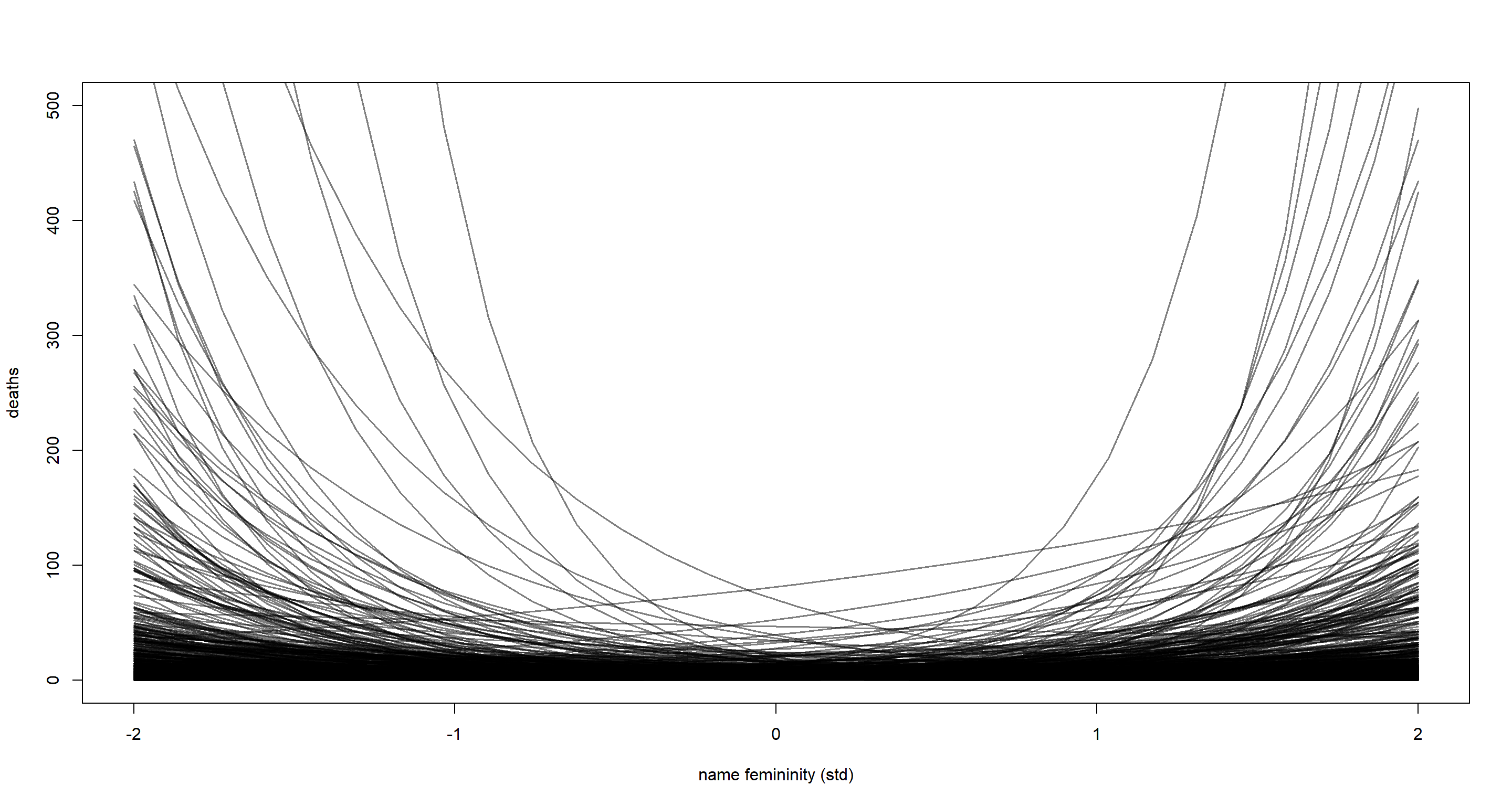
I’d think that’s pretty alright. We allow for both positive and negative trends between death toll and femininity of hurricane name, but don’t have a lot of explosive trends in our priors. These strong trends are quite unintuitive. Our vast majority of trends however are very ambiguous and so I proceed with these priors and run the model:
mH1 <- ulam(f, data = dat, chains = 4, cores = 4, log_lik = TRUE)
precis(mH1)
##         mean         sd      5.5%     94.5%    n_eff     Rhat4
## a  2.9994821 0.02344260 2.9612043 3.0356100 1145.726 0.9982237
## bF 0.2386957 0.02488145 0.1994521 0.2784917 1371.036 0.9996256
So according to this, there is a positive relationship between hurricane name femininity and death toll. Which hurricanes do we actually retrodict well, though? Let’s plot, this:
# plot raw data
plot(dat$F, dat$D,
  pch = 16, lwd = 2,
  col = rangi2, xlab = "femininity (std)", ylab = "deaths"
)
# compute model-based trend
pred_dat <- list(F = seq(from = -2, to = 2, length.out = 1e2))
lambda <- link(mH1, data = pred_dat) # predict deaths
lambda.mu <- apply(lambda, 2, mean) # get mean prediction
lambda.PI <- apply(lambda, 2, PI) # get prediction interval
# superimpose trend
lines(pred_dat$F, lambda.mu)
shade(lambda.PI, pred_dat$F)
# compute sampling distribution
deaths_sim <- sim(mH1, data = pred_dat) # simulate posterior observations
deaths_sim.PI <- apply(deaths_sim, 2, PI) # get simulation interval
# superimpose sampling interval as dashed lines
lines(pred_dat$F, deaths_sim.PI[1, ], lty = 2)
lines(pred_dat$F, deaths_sim.PI[2, ], lty = 2)
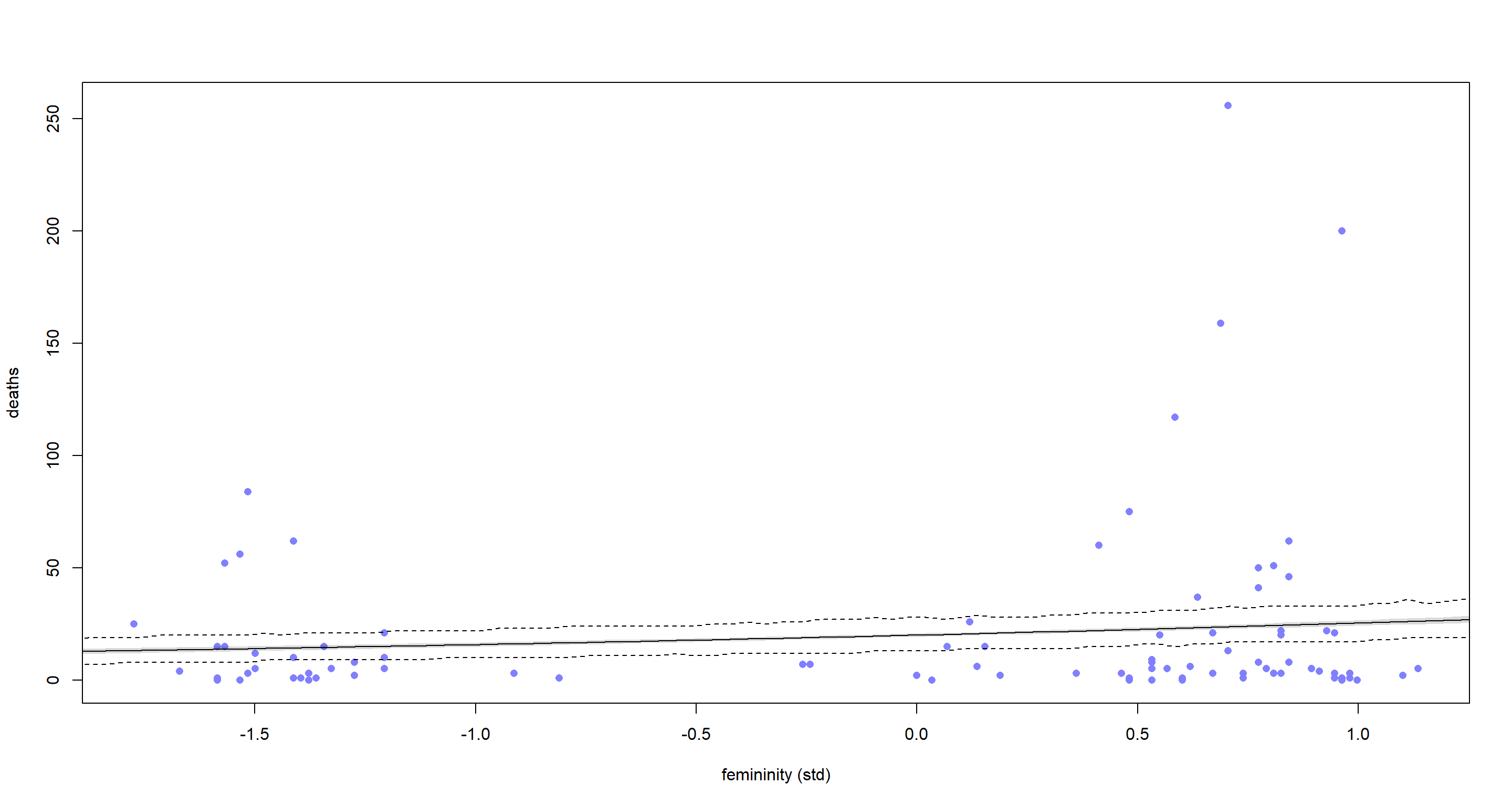
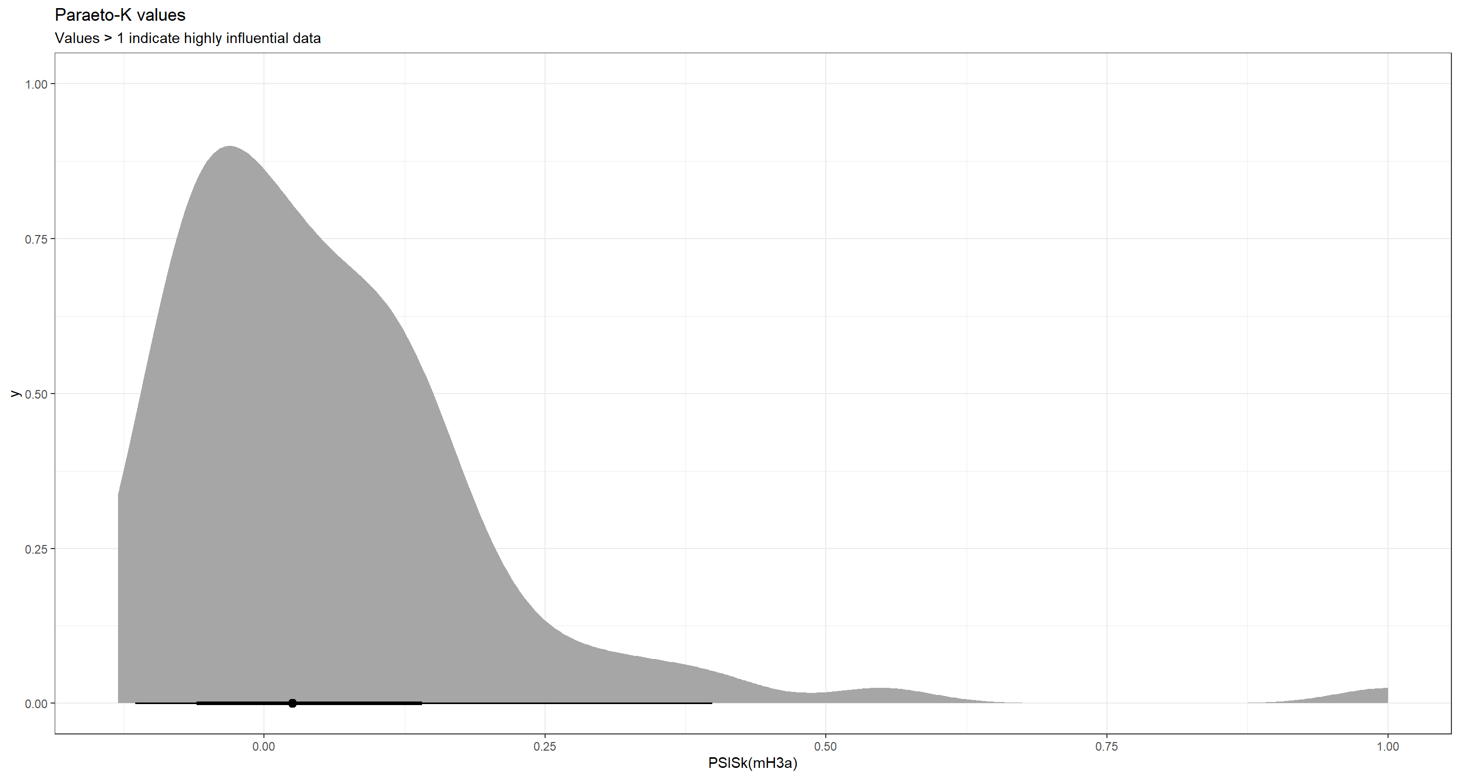
Ok. There is quite a bit to unpack here. First of all, our model does not retrodict many of the hurricanes well even though it is quite certain of its predictions (grey shaded area which is hardly visible). Quite obviously, this model misses many of the hurricane death tolls to the right hand side of the above plot. This is a clear sign of over-dispersion which our model failed to account for. The weak, positive trend we are seeing here seems to be informed largely by these highly influential data points. We can assess whether and how influential some data points are with the Paraeto-K values (anything above 1 indicates an influential data point) following:
ggplot(as.data.frame(PSISk(mH1)), aes(x = PSISk(mH1))) +
  stat_halfeye() +
  theme_bw() +
  labs(title = "Paraeto-K values", subtitle = "Values > 1 indicate highly influential data")
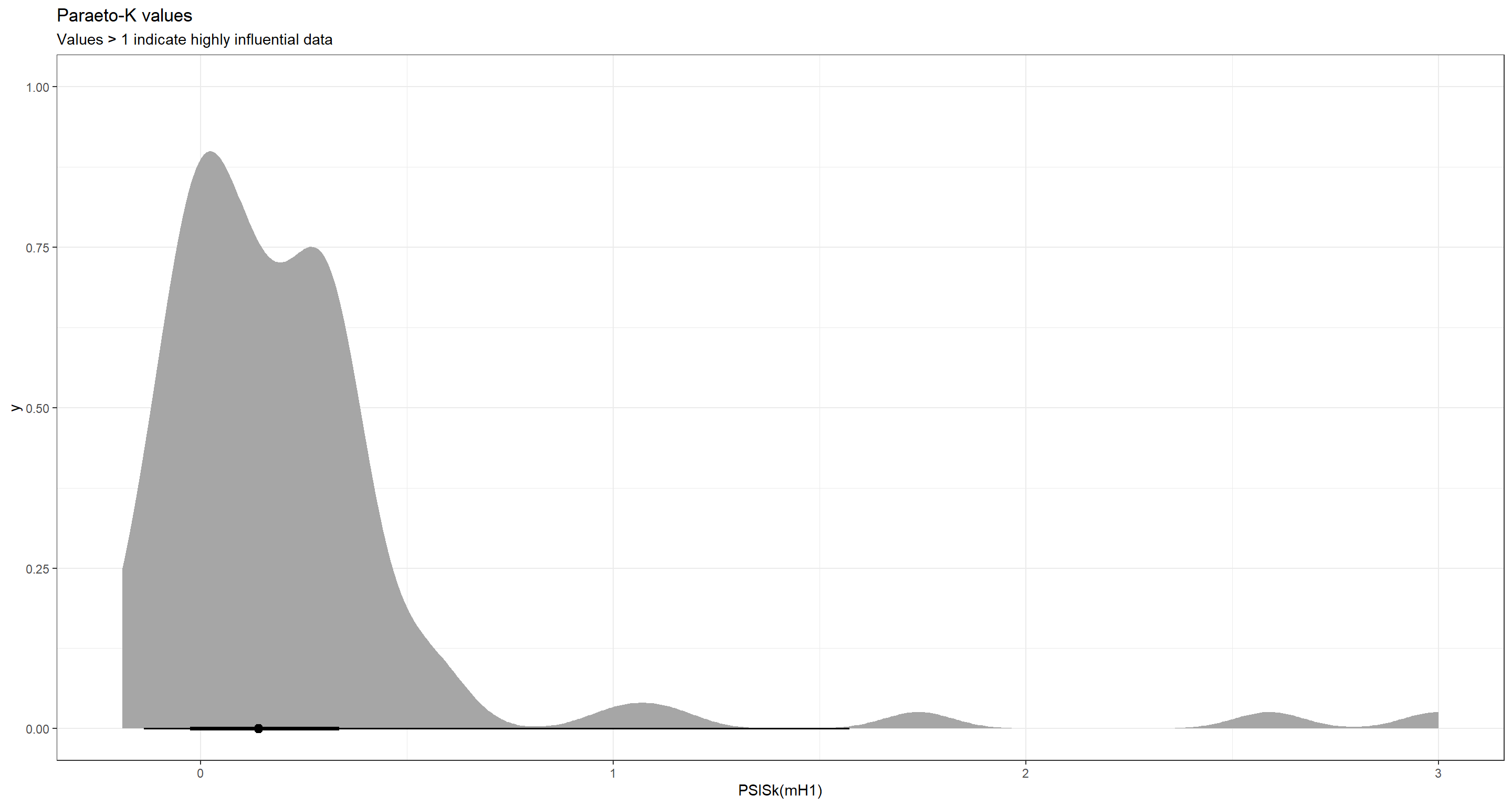
Boy! Some hurricanes really do drive our model to a big extent!
Practice H2
Question: Counts are nearly always over-dispersed relative to Poisson. So fit a gamma-Poisson (aka negative-binomial) model to predict deaths using femininity. Show that the over-dispersed model no longer shows as precise a positive association between femininity and deaths, with an 89% interval that overlaps zero. Can you explain why the association diminished in strength?
Answer: To start this off, I load the library and data again, so much of the exercise and my solutions can stand by itself:
library(rethinking)
data(Hurricanes)
d <- Hurricanes # load data on object called d
d$fem_std <- (d$femininity - mean(d$femininity)) / sd(d$femininity) # standardised femininity
dat <- list(D = d$deaths, F = d$fem_std)
Again, with the data prepared, we fit our model - the same model as before just with a different outcome distribution:
mH2 <- ulam(
  alist(
    D ~ dgampois(lambda, scale),
    log(lambda) <- a + bF * F,
    a ~ dnorm(1, 1),
    bF ~ dnorm(0, 1),
    scale ~ dexp(1) # strictly positive hence why exponential prior
  ),
  data = dat, chains = 4, cores = 4, log_lik = TRUE
)
precis(mH2)
##            mean         sd        5.5%     94.5%    n_eff     Rhat4
## a     2.9780290 0.15272205  2.73722408 3.2334449 1908.835 0.9989114
## bF    0.2107239 0.15442227 -0.04075382 0.4566408 1737.246 0.9993676
## scale 0.4532751 0.06226293  0.35889278 0.5579919 1897.214 1.0003374
Cool. Our previously identified positive relationship between standardised femininity of hurricane name and death toll is still there albeit slightly diminished in magnitude. However, the credible interval around it has widened considerably and overlaps zero now.
Let’s compare the estimates of our models side by side:
plot(coeftab(mH1, mH2))
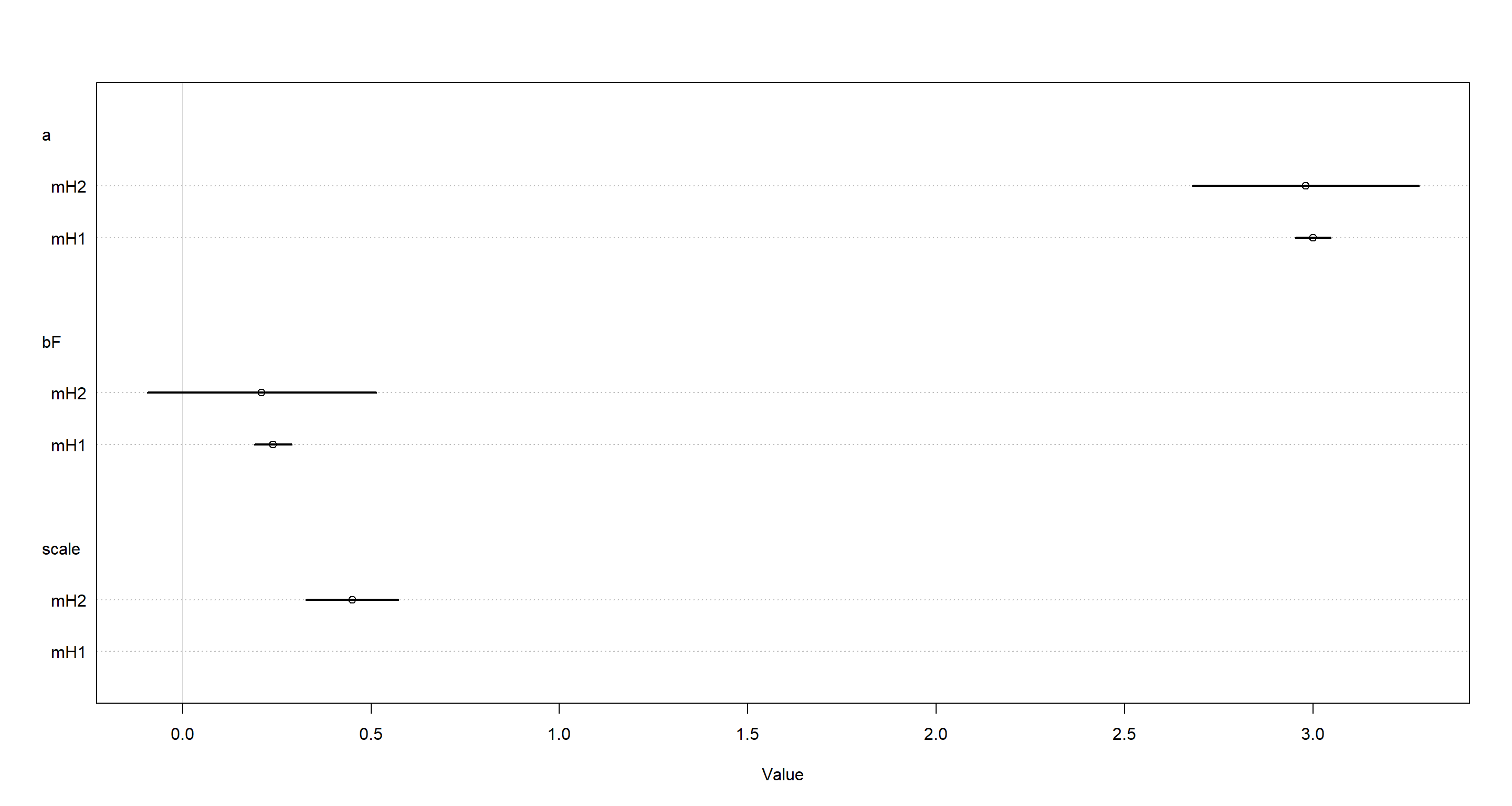
These shows quite clearly how our new model is much more uncertain of the parameters.
So what about the predictions of this new model? I plot them the exact same way as previously:
# plot raw data
plot(dat$F, dat$D,
  pch = 16, lwd = 2,
  col = rangi2, xlab = "femininity (std)", ylab = "deaths"
)
# compute model-based trend
pred_dat <- list(F = seq(from = -2, to = 2, length.out = 1e2))
lambda <- link(mH2, data = pred_dat)
lambda.mu <- apply(lambda, 2, mean)
lambda.PI <- apply(lambda, 2, PI)
# superimpose trend
lines(pred_dat$F, lambda.mu)
shade(lambda.PI, pred_dat$F)
# compute sampling distribution
deaths_sim <- sim(mH2, data = pred_dat)
deaths_sim.PI <- apply(deaths_sim, 2, PI)
# superimpose sampling interval as dashed lines
lines(pred_dat$F, deaths_sim.PI[1, ], lty = 2)
lines(pred_dat$F, deaths_sim.PI[2, ], lty = 2)
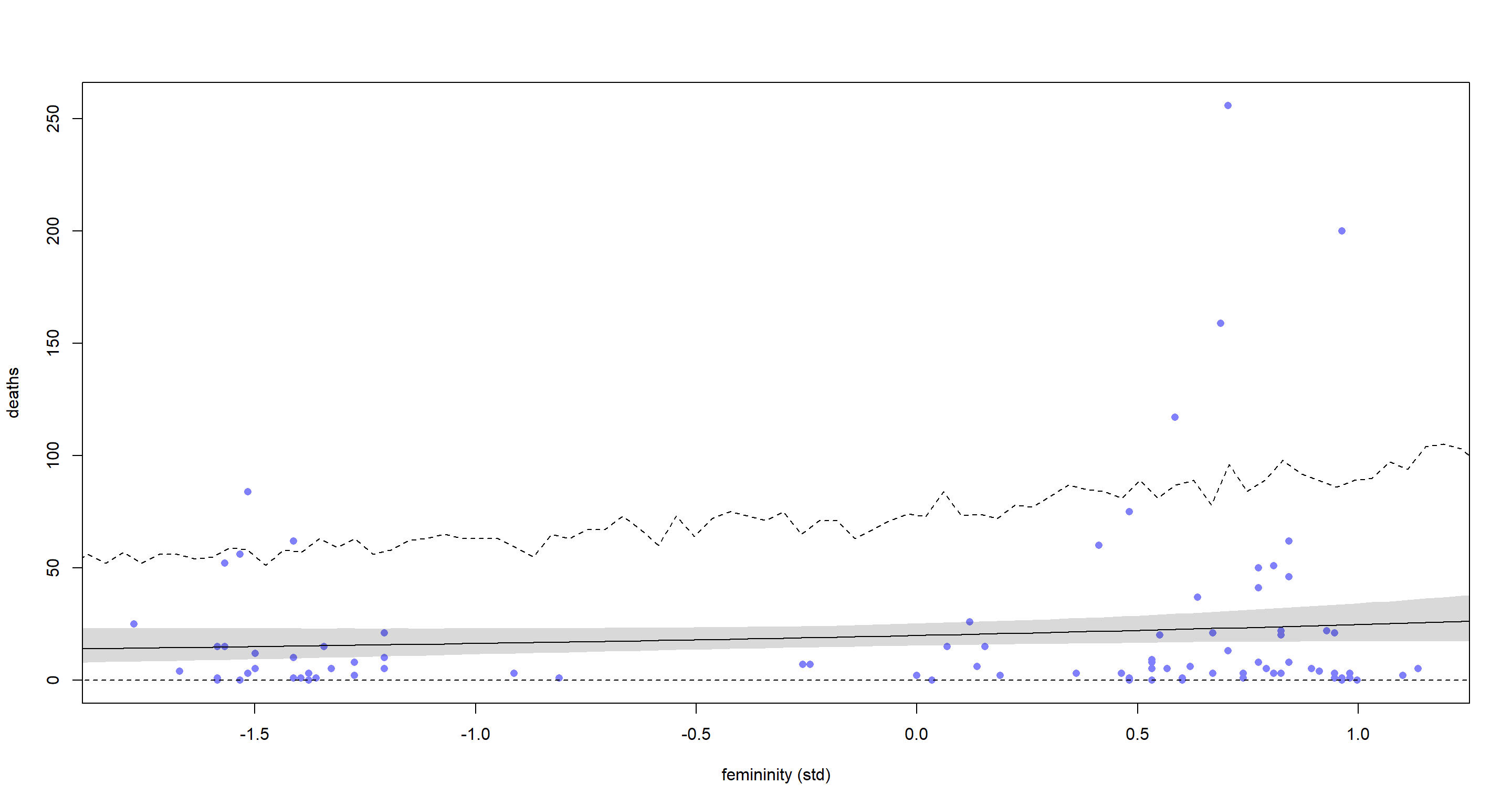 What’s there left to say other than: “Look at that increased uncertainty of our model” at this point? Well, we can talk about the accuracy of our predictions. They still blow. The uncertainty of our model is nice and all, but with a predictive accuracy like this why would we trust the model?
For now, let’s turn to the conceptual part of this exercise: “Why has the association diminished with the new model?” The question comes down to understanding what the gamma distribution does to our model. The gamma distribution allows for a death rate to be calculated for each outcome individually rather than one overall death rate for all hurricanes. These individual rates are sampled from a common distribution which is a function of the femininity of hurricane names. As a matter of fact, we can plot this:
post <- extract.samples(mH2)
par(mfrow = c(1, 3))
for (fem in -1:1) {
  for (i in 1:1e2) {
    curve(dgamma2(
      x, # where to calculate density
      exp(post$a[i] + post$bF[i] * fem), # linear model with inverse link applied
      post$scale[i] # scale for gamma
    ),
    from = 0, to = 70, xlab = "mean deaths", ylab = "Density",
    ylim = c(0, 0.19), col = col.alpha("black", 0.2),
    add = ifelse(i == 1, FALSE, TRUE)
    )
  }
  mtext(concat("femininity  =   ", fem))
}
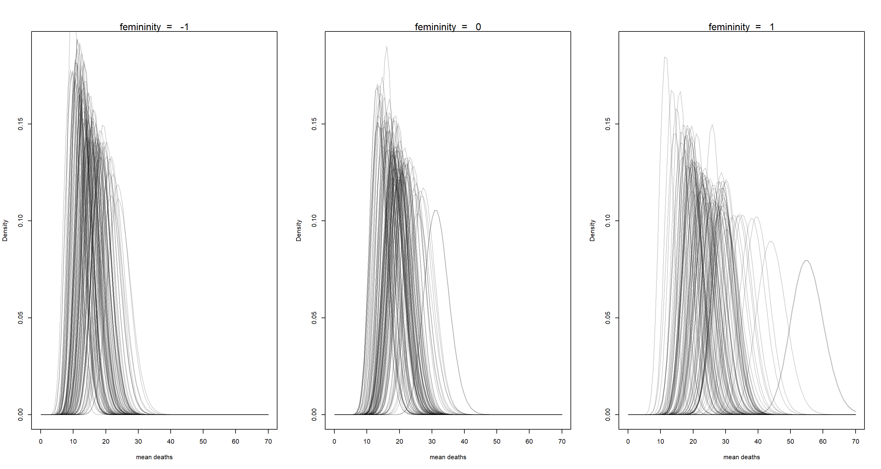
These are the gamma distributions samples from the posterior distribution of death rates when assuming same femininity of name for all of them at three different levels of femininity. Yes, a distribution sampled from another distribution. The above plots simply show the uncertainty of which gamma distribution to settle on.
Since our model and gamma distributions are informed by a, bF, and the scale for the gamma distribution at the same time many combinations of a and bF are consistent with the data which results in a wider posterior distribution.
Finally, let’s look at Paraeto-K values and potentially influential data again:
ggplot(as.data.frame(PSISk(mH2)), aes(x = PSISk(mH2))) +
  stat_halfeye() +
  theme_bw() +
  labs(title = "Paraeto-K values", subtitle = "Values > 1 indicate highly influential data")
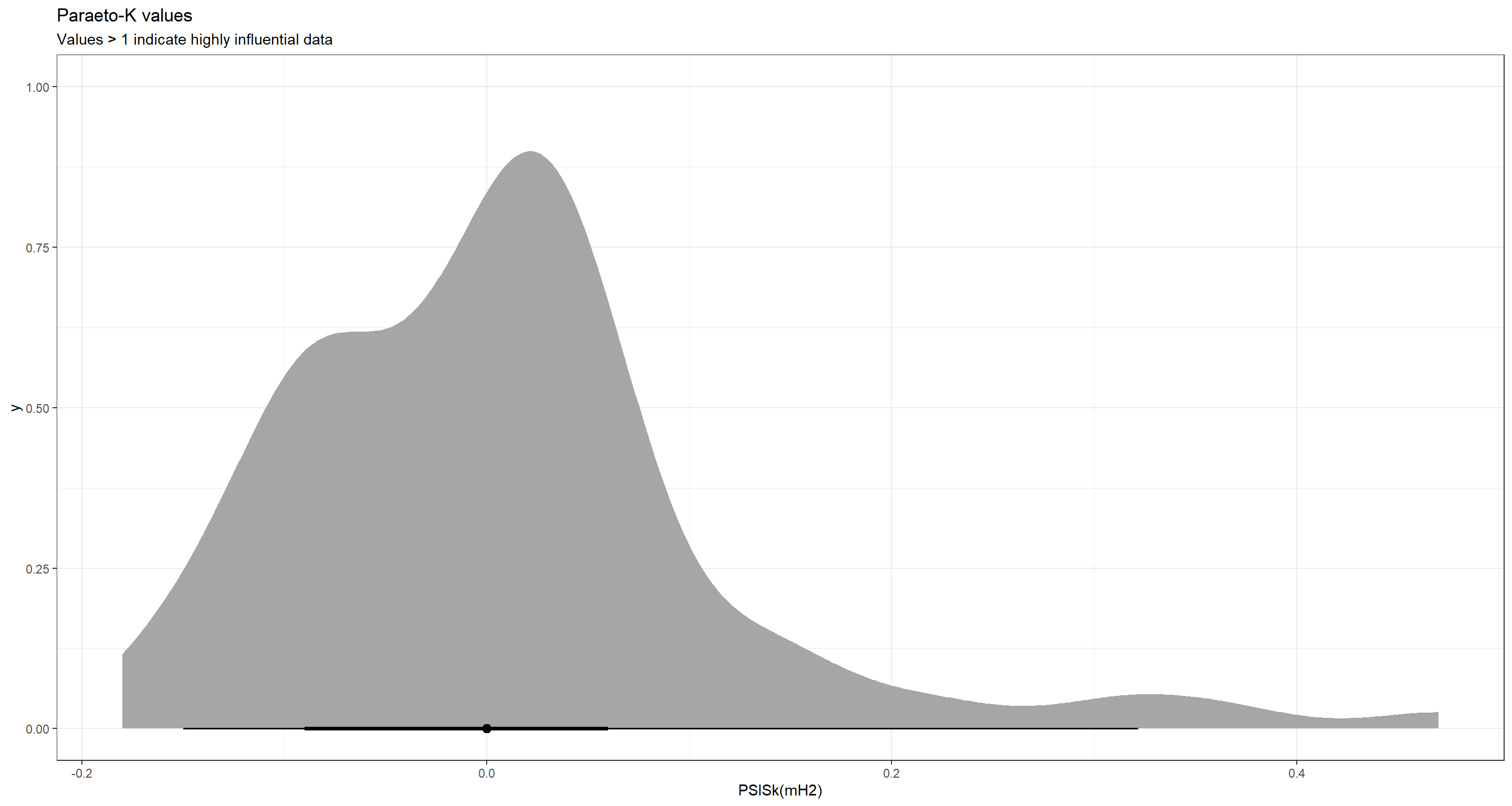
MUCH BETTER than before!
Practice H3
Question: In order to infer a strong association between deaths and femininity, it’s necessary to include an interaction effect. In the data, there are two measures of a hurricane’s potential to cause death: damage_norm and min_pressure. Consult ?Hurricanes for their meanings. It makes some sense to imagine that femininity of a name matters more when the hurricane is itself deadly. This implies an interaction between femininity and either or both of damage_norm and min_pressure. Fit a series of models evaluating these interactions. Interpret and compare the models. In interpreting the estimates, it may help to generate counterfactual predictions contrasting hurricanes with masculine and feminine names. Are the effect sizes plausible?
Answer: To start this off, I load the library and data again, so much of the exercise and my solutions can stand by itself:
library(rethinking)
data(Hurricanes)
d <- Hurricanes # load data on object called d
d$fem_std <- (d$femininity - mean(d$femininity)) / sd(d$femininity) # standardised femininity
dat <- list(D = d$deaths, F = d$fem_std)
dat$P <- standardize(d$min_pressure)
dat$S <- standardize(d$damage_norm)
The data is ready and I step into my model fitting procedure. Here, I start with a basic model which builds on the previous gamma-Poisson model by adding an interaction between femininity and min_pressure:
mH3a <- ulam(
  alist(
    D ~ dgampois(lambda, scale),
    log(lambda) <- a + bF * F + bP * P + bFP * F * P,
    a ~ dnorm(1, 1),
    c(bF, bP, bFP) ~ dnorm(0, 1),
    scale ~ dexp(1)
  ),
  data = dat, cores = 4, chains = 4, log_lik = TRUE
)
precis(mH3a)
##             mean         sd        5.5%      94.5%    n_eff     Rhat4
## a      2.7499528 0.13739615  2.53479738  2.9731015 2057.085 0.9990744
## bFP    0.2991240 0.14883183  0.06678460  0.5242145 1849.512 1.0007366
## bP    -0.6715712 0.13597028 -0.88624645 -0.4539281 1894.311 1.0002580
## bF     0.3027293 0.14148646  0.08381879  0.5332170 1953.726 0.9999575
## scale  0.5523986 0.08078761  0.42818191  0.6867295 1985.855 0.9987496
As minimum pressure gets lower, a storm grows stronger (I was confused by that myself when answering these exercises). Quite obviously, the lower the pressure in a storm, the more severe the storm, and the more people die which is reflected by the negative value in bP. bF is still estimated to be positive. This time, the interval doesn’t even overlap zero. Meanwhile, the interaction effect bFP is positive. I find it hard to interpret this so I’d rather plot some predictions against real data:
P_seq <- seq(from = -3, to = 2, length.out = 1e2) # pressure sequence
# 'masculine' storms
d_pred <- data.frame(F = -1, P = P_seq)
lambda_m <- link(mH3a, data = d_pred)
lambda_m.mu <- apply(lambda_m, 2, mean)
lambda_m.PI <- apply(lambda_m, 2, PI)
# 'feminine' storms
d_pred <- data.frame(F = 1, P = P_seq)
lambda_f <- link(mH3a, data = d_pred)
lambda_f.mu <- apply(lambda_f, 2, mean)
lambda_f.PI <- apply(lambda_f, 2, PI)
# Plotting, sqrt() to make differences easier to spot, can't use log because there are storm with zero deaths
plot(dat$P, sqrt(dat$D),
  pch = 1, lwd = 2, col = ifelse(dat$F > 0, "red", "dark gray"),
  xlab = "minimum pressure (std)", ylab = "sqrt(deaths)"
)
lines(P_seq, sqrt(lambda_m.mu), lty = 2)
shade(sqrt(lambda_m.PI), P_seq)
lines(P_seq, sqrt(lambda_f.mu), lty = 1, col = "red")
shade(sqrt(lambda_f.PI), P_seq, col = col.alpha("red", 0.2))
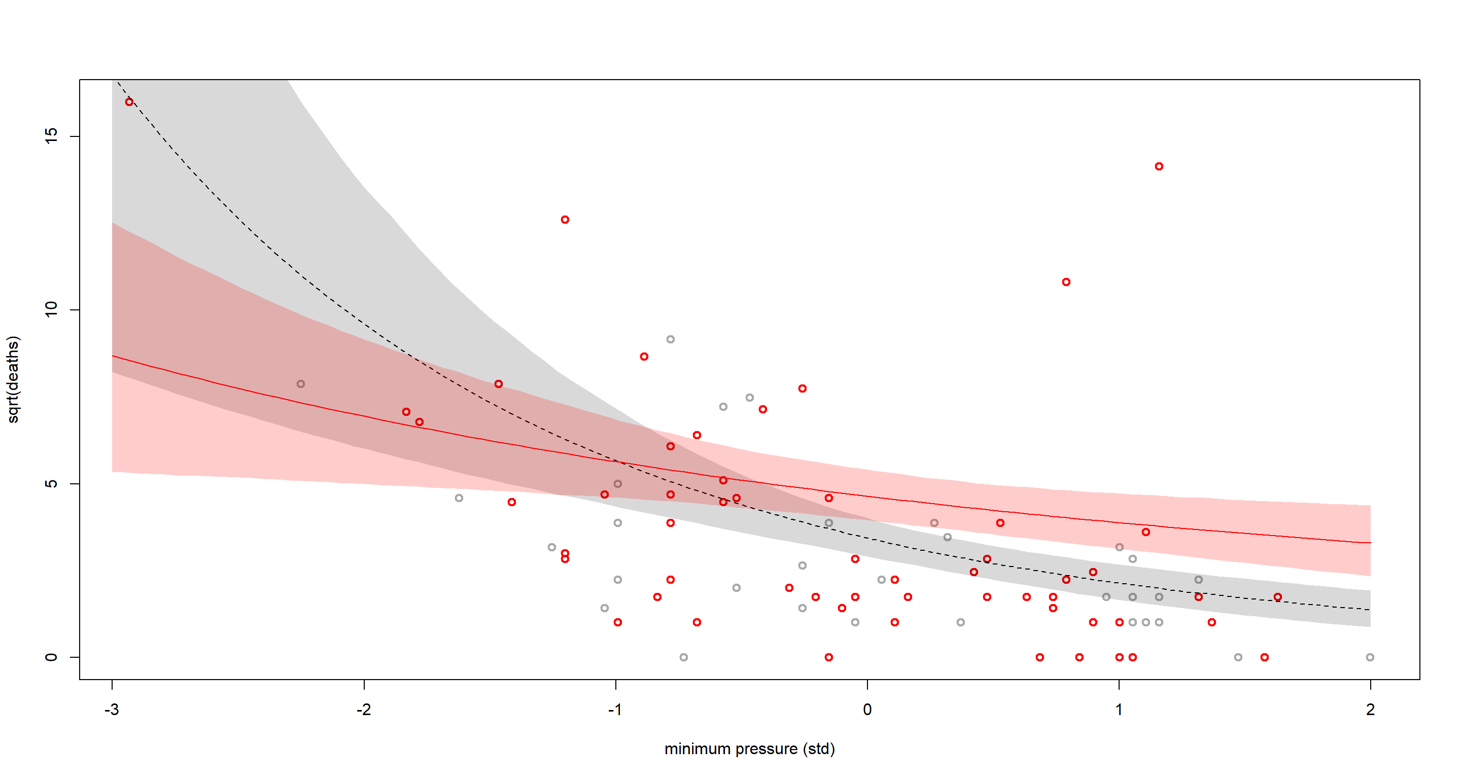
Our model expects masculine (grey) storms to be less deadly, on average, than feminine (red) ones. As pressure drops (toward the rightward side of the plot above), these differences become smaller and smaller. Quite evidently, some of these storms are influencing what our model predicts much more so than others:
ggplot(as.data.frame(PSISk(mH3a)), aes(x = PSISk(mH3a))) +
  stat_halfeye() +
  theme_bw() +
  labs(title = "Paraeto-K values", subtitle = "Values > 1 indicate highly influential data")
Let’s turn to the second variable we may want to add damage_norm - the damage caused by each storm:
mH3b <- ulam(
  alist(
    D ~ dgampois(lambda, scale),
    log(lambda) <- a + bF * F + bS * S + bFS * F * S,
    a ~ dnorm(1, 1),
    c(bF, bS, bFS) ~ dnorm(0, 1),
    scale ~ dexp(1)
  ),
  data = dat, chains = 4, cores = 4, log_lik = TRUE
)
precis(mH3b)
##             mean         sd        5.5%     94.5%    n_eff     Rhat4
## a     2.56677402 0.12946975  2.36261687 2.7748946 1903.061 0.9995145
## bFS   0.30853835 0.20499020 -0.04173134 0.6265386 2243.101 0.9994129
## bS    1.25058627 0.21057791  0.92538673 1.5951083 1956.116 1.0003102
## bF    0.08485749 0.12501328 -0.11660977 0.2820823 1963.489 1.0005148
## scale 0.68529101 0.09803179  0.53525802 0.8466209 2165.010 0.9990485
That just eradicated the effect of femininity of hurricane name (bF)! The newly added interaction parameter bFS is incredibly strong and positive. Again, let’s visualise this:
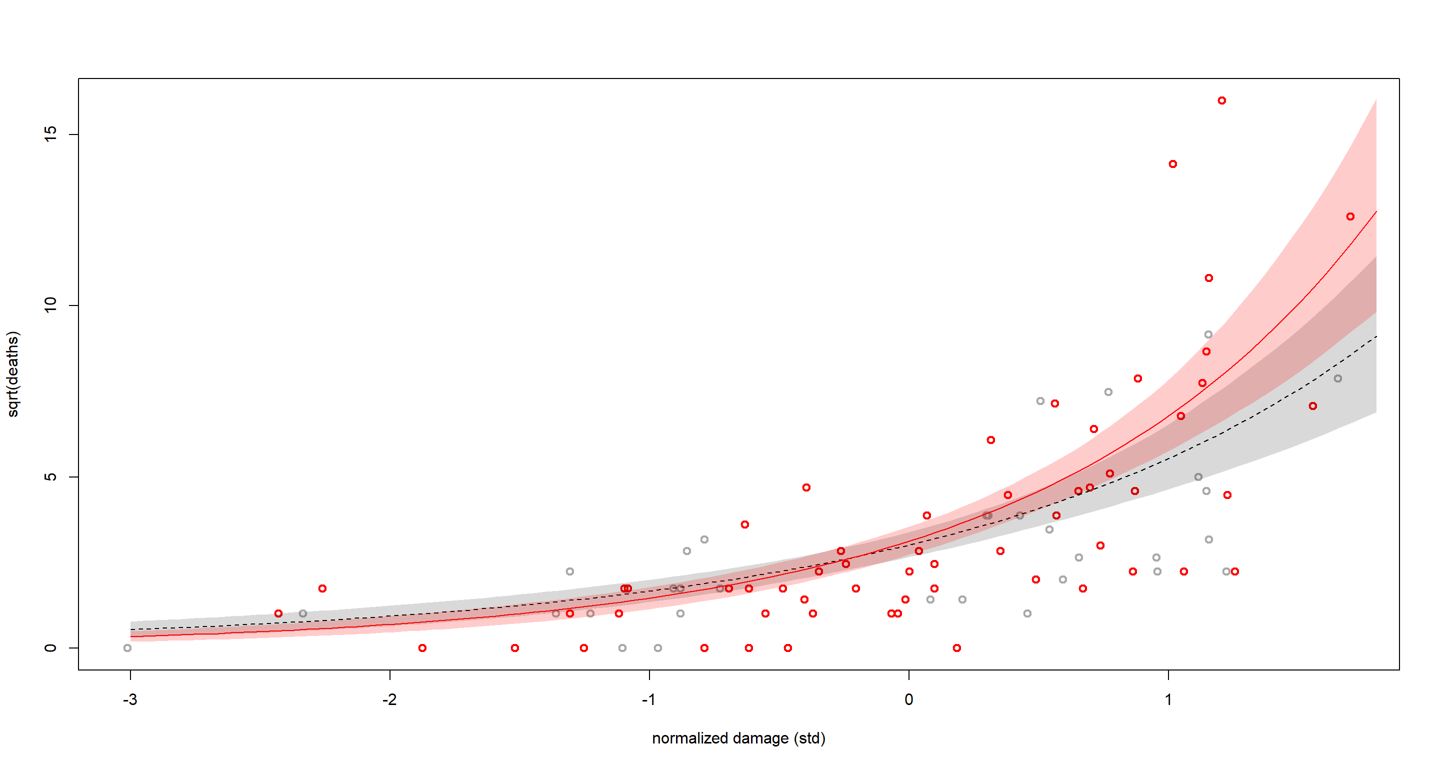
S_seq <- seq(from = -1, to = 5.5, length.out = 1e2) # damage sequence
# 'masculine' storms
d_pred <- data.frame(F = -1, S = S_seq)
lambda_m <- link(mH3b, data = d_pred)
lambda_m.mu <- apply(lambda_m, 2, mean)
lambda_m.PI <- apply(lambda_m, 2, PI)
# 'feminine' storms
d_pred <- data.frame(F = 1, S = S_seq)
lambda_f <- link(mH3b, data = d_pred)
lambda_f.mu <- apply(lambda_f, 2, mean)
lambda_f.PI <- apply(lambda_f, 2, PI)
# plot
plot(dat$S, sqrt(dat$D),
  pch = 1, lwd = 2, col = ifelse(dat$F > 0, "red", "dark gray"),
  xlab = "normalized damage (std)", ylab = "sqrt(deaths)"
)
lines(S_seq, sqrt(lambda_m.mu), lty = 2)
shade(sqrt(lambda_m.PI), S_seq)
lines(S_seq, sqrt(lambda_f.mu), lty = 1, col = "red")
shade(sqrt(lambda_f.PI), S_seq, col = col.alpha("red", 0.2))
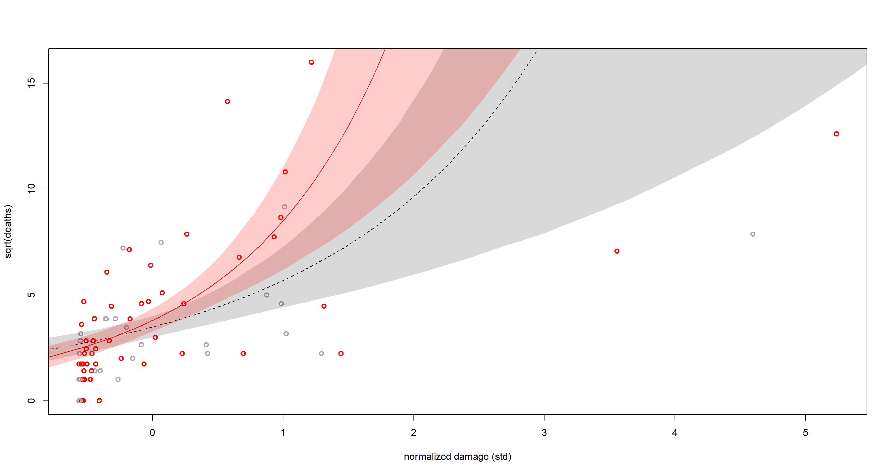
We can clearly see how our model makes less of a distinction between masculine and feminine hurricanes overall at this point. Damage norm scales multiplicatively. The distances grow fast as we approach the rightward side of the plot. This is difficult for the model to account for. Hence why the model is underwhelming.
So why is the interaction effect so strong? Probably because of those 3-4 highly influential feminine storms at the upper-righthand corner of our plot above which implies that feminine storms are especially deadly when they are damaging to begin with. Personally, I don’t trust this association and would argue that there is no logical reason for it and most likely an artefact of the limited data availability.
Practice H4
Question: In the original hurricanes paper, storm damage (damage_norm) was used directly. This assumption implies that mortality increases exponentially with a linear increase in storm strength, because a Poisson regression uses a log link. So it’s worth exploring an alternative hypothesis: that the logarithm of storm strength is what matters. Explore this by using the logarithm of damage_norm as a predictor. Using the best model structure from the previous problem, compare a model that uses log(damage_norm) to a model that uses damage_norm directly. Compare their DIC/WAIC values as well as their implied predictions. What do you conclude?
Answer: To start this off, I load the library and data again, so much of the exercise and my solutions can stand by itself:
library(rethinking)
data(Hurricanes)
d <- Hurricanes # load data on object called d
d$fem_std <- (d$femininity - mean(d$femininity)) / sd(d$femininity) # standardised femininity
dat <- list(D = d$deaths, F = d$fem_std)
dat$S2 <- standardize(log(d$damage_norm))
Let’s fit the model as before and compare it to the previously identified best model:
mH4 <- ulam(
  alist(
    D ~ dgampois(lambda, scale),
    log(lambda) <- a + bF * F + bS * S2 + bFS * F * S2,
    a ~ dnorm(1, 1),
    c(bF, bS, bFS) ~ dnorm(0, 1),
    scale ~ dexp(1)
  ),
  data = dat, chains = 4, cores = 4, log_lik = TRUE
)
compare(mH3b, mH4, func = PSIS)
##          PSIS       SE    dPSIS      dSE    pPSIS       weight
## mH4  630.7019 31.19102  0.00000       NA 5.376913 1.000000e+00
## mH3b 670.6361 34.19897 39.93425 13.67922 6.857192 2.130043e-09
Model mH4 clearly outperforms the earlier (non-logarithmic) model mH3b. How do the parameter estimates look in comparison?
plot(coeftab(mH3b, mH4),
  labels = paste(rep(rownames(coeftab(mH3b, mH4)@coefs), each = 2),
    rep(c("Norm", "Log"), nrow(coeftab(mH3b, mH4)@coefs) * 2),
    sep = "-"
  )
)
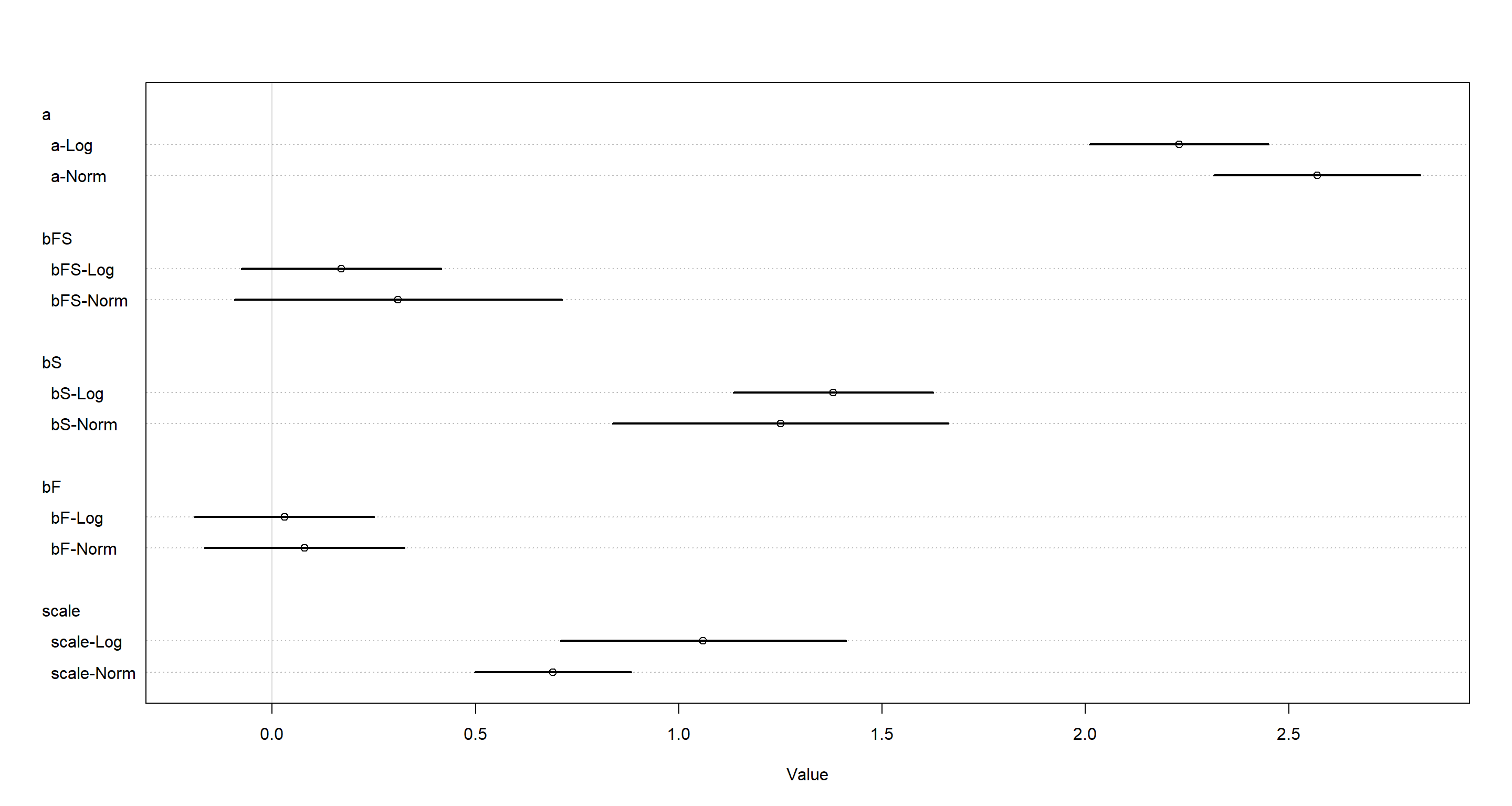
With the log-transformed input, bFS has increased in magnitude. What do the resulting predictions look like?
S2_seq <- seq(from = -3, to = 1.8, length.out = 1e2)
# 'masculine' storms
d_pred <- data.frame(F = -1, S2 = S2_seq)
lambda_m <- link(mH4, data = d_pred)
lambda_m.mu <- apply(lambda_m, 2, mean)
lambda_m.PI <- apply(lambda_m, 2, PI)
# 'feminine' storms
d_pred <- data.frame(F = 1, S2 = S2_seq)
lambda_f <- link(mH4, data = d_pred)
lambda_f.mu <- apply(lambda_f, 2, mean)
lambda_f.PI <- apply(lambda_f, 2, PI)
# plot
plot(dat$S2, sqrt(dat$D),
  pch = 1, lwd = 2, col = ifelse(dat$F > 0, "red", "dark gray"),
  xlab = "normalized damage (std)", ylab = "sqrt(deaths)"
)
lines(S2_seq, sqrt(lambda_m.mu), lty = 2)
shade(sqrt(lambda_m.PI), S2_seq)
lines(S2_seq, sqrt(lambda_f.mu), lty = 1, col = "red")
shade(sqrt(lambda_f.PI), S2_seq, col = col.alpha("red", 0.2))
Now this model fits the data much better! Still not perfect, but much better.
Practice H5
Question: One hypothesis from developmental psychology, usually attributed to Carol Gilligan, proposes that women and men have different average tendencies in moral reasoning. Like most hypotheses in social psychology, it is merely descriptive. The notion is that women are more concerned with care (avoiding harm), while men are more concerned with justice and rights. Culture-bound nonsense? Yes. Descriptively accurate? Maybe.
Evaluate this hypothesis, using the Trolley data, supposing that contact provides a proxy for physical harm. Are women more or less bothered by contact than are men, in these data? Figure out the model(s) that is needed to address this question.
Answer: Again, let’s start by preparing the data:
library(rethinking)
data(Trolley)
d <- Trolley
dat <- list(
  R = d$response,
  A = d$action,
  I = d$intention,
  C = d$contact
)
dat$Gid <- ifelse(d$male == 1, 1L, 2L)
Now for a model. We use the same model skeleton as provided in the book. However, this time around, we want cutpoints in our ordered, cumulative logit for both genders separately:
dat$F <- 1L - d$male # indicator of femaleness to turn intercepts on and off
mH5 <- ulam(
  alist(
    R ~ dordlogit(phi, cutpoints),
    phi <- a * F + bA[Gid] * A + bC[Gid] * C + BI * I,
    BI <- bI[Gid] + bIA[Gid] * A + bIC[Gid] * C,
    c(bA, bI, bC, bIA, bIC)[Gid] ~ dnorm(0, 0.5),
    a ~ dnorm(0, 0.5),
    cutpoints ~ dnorm(0, 1.5)
  ),
  data = dat, chains = 4, cores = 4
)
precis(mH5, depth = 2)
##                     mean         sd        5.5%       94.5%     n_eff    Rhat4
## bIC[1]       -1.29000860 0.13002100 -1.50109161 -1.07614615 1348.3365 1.000146
## bIC[2]       -1.14842366 0.13434342 -1.36319985 -0.93345115 1163.2537 1.006455
## bIA[1]       -0.43821462 0.10411766 -0.60427628 -0.27043071 1201.4372 1.003107
## bIA[2]       -0.42253949 0.11300405 -0.59891439 -0.23526558 1156.5531 1.005345
## bC[1]        -0.47691217 0.09253044 -0.62813726 -0.32838280 1294.9094 1.000744
## bC[2]        -0.20730657 0.09595489 -0.36193206 -0.06036975 1207.3517 1.004505
## bI[1]        -0.33520753 0.07772555 -0.46098056 -0.20740598 1075.2158 1.003142
## bI[2]        -0.25819201 0.08096287 -0.39036524 -0.12766901 1026.1192 1.006898
## bA[1]        -0.59363382 0.07036947 -0.70451058 -0.48492259 1075.2269 1.005641
## bA[2]        -0.33605523 0.07724757 -0.45859501 -0.21053675 1205.2000 1.005800
## a            -0.78364935 0.08006100 -0.90628106 -0.65659045  948.2152 1.003790
## cutpoints[1] -3.02124197 0.06328453 -3.11858791 -2.91868150 1181.9794 1.002080
## cutpoints[2] -2.32745650 0.06074323 -2.42260517 -2.23098876 1175.2672 1.001935
## cutpoints[3] -1.72766666 0.05885444 -1.82181068 -1.63431341 1123.8787 1.002648
## cutpoints[4] -0.67165728 0.05700586 -0.76381567 -0.58315767 1112.3527 1.003052
## cutpoints[5]  0.01889978 0.05633424 -0.07146169  0.10708376 1122.8518 1.003504
## cutpoints[6]  0.94926239 0.05853165  0.85602268  1.04283590 1166.1198 1.002682
The parameter estimates of interest here are:
a(-0.78) - main effect of being female on cumulative log-odds. On average women, have more moral qualms about the trolley problem it seems.bC[2](-0.21) - the interaction effect of being both female and in a contact scenario as opposed tobc[1](-0.48) which is the same scenario but for men. Women in our set-up had less moral issues with contact events.
The latter goes against the previously stated hypothesis. Why is that? Because the people in our study are much more complex than just their genders.
Practice H6
Question: The data in data(Fish) are records of visits to a national park. See ?Fish for details. The question of interest is how many fish an average visitor takes per hour, when fishing. The problem is that not everyone tried to fish, so the fish_caught numbers are zero-inflated. As with the monks example in the chapter, there is a process that determines who is fishing (working) and another process that determines fish per hour (manuscripts per day), conditional on fishing (working). We want to model both. Otherwise we’ll end up with an underestimate of rate of fish extraction from the park.
You will model these data using zero-inflated Poisson GLMs. Predict fish_caught as a function
of any of the other variables you think are relevant. One thing you must do, however, is use a proper Poisson offset/exposure in the Poisson portion of the zero-inflated model. Then use the hours variable to construct the offset. This will adjust the model for the differing amount of time individuals spent in the park.
Answer: One last time, for this week, we prepare some data:
library(rethinking)
data(Fish)
d <- Fish
str(d)
## 'data.frame':	250 obs. of  6 variables:
##  $ fish_caught: int  0 0 0 0 1 0 0 0 0 1 ...
##  $ livebait   : int  0 1 1 1 1 1 1 1 0 1 ...
##  $ camper     : int  0 1 0 1 0 1 0 0 1 1 ...
##  $ persons    : int  1 1 1 2 1 4 3 4 3 1 ...
##  $ child      : int  0 0 0 1 0 2 1 3 2 0 ...
##  $ hours      : num  21.124 5.732 1.323 0.548 1.695 ...
The model I want to build will look at the following variables:
fish_caught. This is our response variable.livebait. I suggest that using livebait increases number of fish caught.camper. I assume that being a camper increases the chances that one goes fishing, but not necessarily the number of fish caught.persons. I assume that the number of people in a group increases how many fish are caught.child. Being a child should reasonably determine both whether one fishes (I assume children fish less - call it personal bias) and also that they are less effective than adults.hours. How long one fishes surely determines how many fish are caught. I want to include the base rate of these into my model of fish caught. Since said model will be log-linked, I log-transform them.
Let me fit that model:
d$loghours <- log(d$hours)
mH6 <- ulam(
  alist(
    # outcome distribution
    fish_caught ~ dzipois(p, mu),
    # linear model for probability of fishing
    logit(p) <- a0 + bC0 * camper + bc0 * child,
    # linear model of catching a number of fish
    log(mu) <- a + bb * livebait + bp * persons + bc * child + bl * loghours,
    c(a0, a) ~ dnorm(0, 1),
    c(bC0, bc0, bb, bp, bc, bl) ~ dnorm(0, 0.5)
  ),
  data = d, chains = 4, cores = 4, log_lik = TRUE
)
precis(mH6)
##           mean         sd       5.5%      94.5%     n_eff     Rhat4
## a   -2.0839466 0.24408479 -2.4814597 -1.6945336  899.9998 1.0016629
## a0  -0.4650216 0.28849629 -0.9436559 -0.0177434 1191.0483 1.0015268
## bl   0.1701858 0.03428906  0.1134792  0.2254237 1255.6829 0.9985511
## bc  -0.8280833 0.10732217 -0.9969186 -0.6569452 1218.3750 1.0024020
## bp   0.8625626 0.04553091  0.7919523  0.9330040 1479.7715 0.9990951
## bb   1.4076543 0.19237711  1.1106049  1.7217943 1169.0384 1.0032455
## bc0  0.9787908 0.23529584  0.6059568  1.3537809 1292.4802 0.9994360
## bC0 -0.6597597 0.29791643 -1.1313113 -0.1803763 1413.3364 1.0017523
Remember that $p$ stands for the probability of not going to fish. Overall, park visitors are pretty likely to fish (a0 =-0.47, logit scale). In line with my intuition, campers are more likely to fish (bC0) while children are less likely to fish (bc0).
Once one is actually fishing, one is not likely to catch much fish (a=-2.08). The parameters pertaining to number of fish caught are expressed on log-scale and so transforming a into the outcome scale (counts of fish) by exponentiating, an adult who fishes by themselves without livebait (this is what a refers to) catches around 0.1249302 fish on average. More people catch more fish (bp). Using livebait is effective (bb). In line with my intuition, children catch less fish than adults (bc). Lastly, the more time one spends fishing, the more fish one catches (bl).
Let’s turn to some actual model predictions of p and mu:
zip_link <- link(mH6)
str(zip_link)
## List of 2
##  $ p : num [1:2000, 1:250] 0.403 0.388 0.469 0.382 0.443 ...
##  $ mu: num [1:2000, 1:250] 0.588 0.543 0.537 0.592 0.488 ...
p cases provide estimates for additional zeros not obtained through the actual Poisson-process behind fishing catches whose output lies with mu.
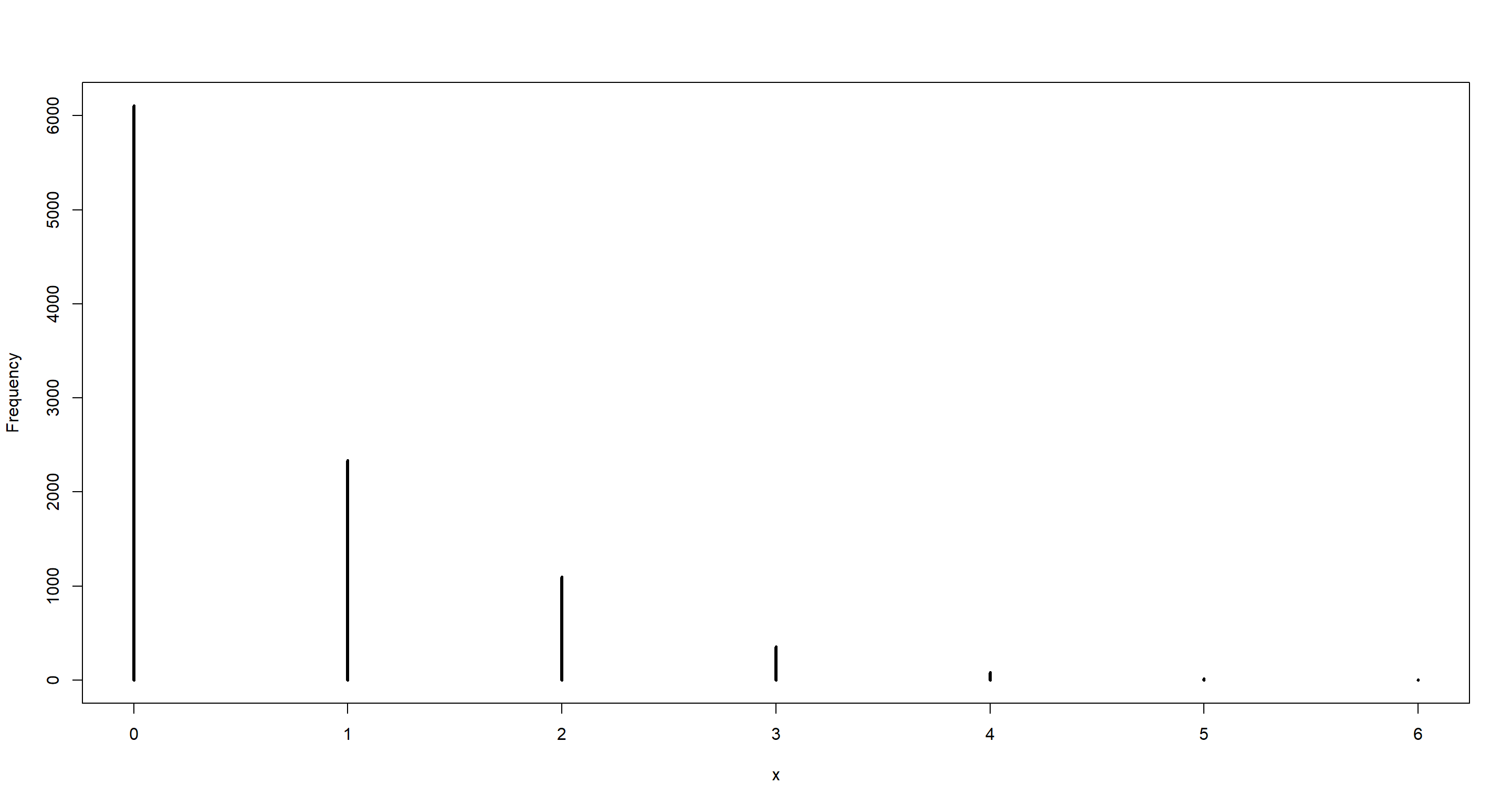
For example, if $p =$0.39 (the inverse logit of a0 in the model above) and $μ = 1$ (much higher than a in the model above for ease here), then the implied predictive distribution is:
zeros <- rbinom(
  n = 1e4, # number of samples
  size = 1,
  prob = inv_logit(precis(mH6)[2, 1]) # probability of going fishing
)
obs_fish <- (1 - zeros) * rpois(1e4, 1)
simplehist(obs_fish)
Let’s see what our model would predict given the estimated parameters:
fish_sim <- sim(mH6)
str(fish_sim)
## num [1:1000, 1:250] 0 0 1 1 0 0 0 2 0 1 ...
This now contains a simulation output for each sample in our data! We could now plot ourselves into oblivion with counterfactual plots. We can also produce counterfactual posterior predictions. As an example, I assume a party of 1 adult spending 1 hour in the park without any use of livebait and not staying the night as a camper:
# new data
pred_dat <- list(
  loghours = log(1), # note that this is zero, the baseline rate
  persons = 1,
  child = 0,
  livebait = 0,
  camper = 0
)
# sim predictions - want expected number of fish, but must use both processes
fish_link <- link(mH6, data = pred_dat)
# summarize
p <- fish_link$p
mu <- fish_link$mu
(expected_fish_mean <- mean((1 - p) * mu))
## [1] 0.1838057
(expected_fish_PI <- PI((1 - p) * mu))
##        5%       94%
## 0.1261989 0.2553580
This tells us that this hypothetical person is expected to catch 0.1838057 fish with the interval displayed above.
Session Info
sessionInfo()
## R version 4.0.5 (2021-03-31)
## Platform: x86_64-w64-mingw32/x64 (64-bit)
## Running under: Windows 10 x64 (build 19043)
##
## Matrix products: default
##
## locale:
## [1] LC_COLLATE=English_United Kingdom.1252  LC_CTYPE=English_United Kingdom.1252    LC_MONETARY=English_United Kingdom.1252 LC_NUMERIC=C
## [5] LC_TIME=English_United Kingdom.1252
##
## attached base packages:
## [1] parallel  stats     graphics  grDevices utils     datasets  methods   base
##
## other attached packages:
## [1] tidybayes_2.3.1      rethinking_2.13      rstan_2.21.2         ggplot2_3.3.6        StanHeaders_2.21.0-7
##
## loaded via a namespace (and not attached):
##  [1] Rcpp_1.0.7           mvtnorm_1.1-1        lattice_0.20-41      tidyr_1.1.3          prettyunits_1.1.1    ps_1.6.0             assertthat_0.2.1     digest_0.6.27        utf8_1.2.1
## [10] V8_3.4.1             plyr_1.8.6           R6_2.5.0             backports_1.2.1      stats4_4.0.5         evaluate_0.14        coda_0.19-4          highr_0.9            blogdown_1.3
## [19] pillar_1.6.0         rlang_0.4.11         curl_4.3.2           callr_3.7.0          jquerylib_0.1.4      R.utils_2.10.1       R.oo_1.24.0          rmarkdown_2.7        styler_1.4.1
## [28] labeling_0.4.2       stringr_1.4.0        loo_2.4.1            munsell_0.5.0        compiler_4.0.5       xfun_0.22            pkgconfig_2.0.3      pkgbuild_1.2.0       shape_1.4.5
## [37] htmltools_0.5.1.1    tidyselect_1.1.0     tibble_3.1.1         gridExtra_2.3        bookdown_0.22        arrayhelpers_1.1-0   codetools_0.2-18     matrixStats_0.61.0   fansi_0.4.2
## [46] crayon_1.4.1         dplyr_1.0.5          withr_2.4.2          MASS_7.3-53.1        R.methodsS3_1.8.1    distributional_0.2.2 ggdist_2.4.0         grid_4.0.5           jsonlite_1.7.2
## [55] gtable_0.3.0         lifecycle_1.0.0      DBI_1.1.1            magrittr_2.0.1       scales_1.1.1         RcppParallel_5.1.2   cli_3.0.0            stringi_1.5.3        farver_2.1.0
## [64] bslib_0.2.4          ellipsis_0.3.2       generics_0.1.0       vctrs_0.3.7          rematch2_2.1.2       forcats_0.5.1        tools_4.0.5          svUnit_1.0.6         R.cache_0.14.0
## [73] glue_1.4.2           purrr_0.3.4          processx_3.5.1       yaml_2.2.1           inline_0.3.17        colorspace_2.0-0     knitr_1.33           sass_0.3.1