Chapter 10 & 11
God Spiked The Integers
Material
Introduction
These are answers and solutions to the exercises at the end of chapter 11 in Satistical Rethinking 2 by Richard McElreath. For anyone reading through these in order and wondering why I skipped chapter 10: chapter 10 did not contain any exercises (to my dismay, as you can imagine). I have created these notes as a part of my ongoing involvement in the AU Bayes Study Group. Much of my inspiration for these solutions, where necessary, has been obtained from Taras Svirskyi, William Wolf, and Corrie Bartelheimer as well as the solutions provided to instructors by Richard McElreath himself.
R Environment
For today’s exercise, I load the following packages:
library(rethinking)
library(rstan)
library(ggplot2)
library(tidybayes)
Easy Exercises
Practice E1
Question: If an event has probability 0.35, what are the log-odds of this event?
Answer: When $p = 0.35$ then the log-odds are $log\frac{0.35}{1-0.35}$, or in R:
log(0.35 / (1 - 0.35))
## [1] -0.6190392
Practice E2
Question: If an event has log-odds 3.2, what is the probability of this event?
Answer: To transform log-odds into probability space, we want to use the inv_logit() function:
inv_logit(3.2)
## [1] 0.9608343
Practice E3
Question: Suppose that a coefficient in a logistic regression has value 1.7. What does this imply about the proportional change in odds of the outcome?
Answer:
exp(1.7)
## [1] 5.473947
Each one-unit increase in the predictor linked to this coefficient results in a multiplication of the odds of the event occurring by 5.47.
The linear model behind the logistic regression simply represents the log-odds of an event happening. The odds of the events happening can thus be shown as $exp(odds)$. Comparing how the odds change when increasing the predictor variable by one unit comes down to solving this equation then:
$$exp(α + βx)Z = exp(α + β(x + 1))$$ Solving this for $z$ results in:
$$z = exp(\beta)$$
which is how we derived the answer to this question.
Practice E4
Question: Why do Poisson regressions sometimes require the use of an offset? Provide an example.
Answer: When study regimes aren’t rigidly standardised, we may end up with count data collected over different time/distance intervals. Comparing these data without accounting for the difference in the underlying sampling frequency will inevitably lead to horribly inadequate predictions of our model(s).
As an example, think of how many ants leave a hive in a certain interval. If we recorded numbers of ants leaving to forage on a minute-by-minute basis, we would obtain much smaller counts than if our sampling regime dictated hourly observation periods. Any poisson model we want to run between differing sampling regimes has to account for the heterogeneity in the observation period lengths. We do so as follows:
$$Ants_i∼Poisson(λ)$$ $$log(λ)=log(period_i)+α+βHive_i$$
Medium Exercises
Practice M1
Question: As explained in the chapter, binomial data can be organized in aggregated and disaggregated forms, without any impact on inference. But the likelihood of the data does change when the data are converted between the two formats. Can you explain why?
Answer: Think back to the Card Drawing Example from chapter 2. We know a certain outcome. Let’s assume two black face, and one white face card are drawn.
In the aggregated form of the data, we obtain the probability of our observation as $3p(1-p)$ (a binomial distribution with $3$ trials and a rate of black face cards of $p = \frac{2}{3}$). This tells us how many ways there are to get two black-face cards out of three pulls of cards. The order is irrelevant.
With disaggregated data, we do not cope with any order, but simply predict the result of each draw of a card by itself and finally multiply our predictions together to form a joint probability according to $p(1-p)$.
In conclusion, aggregated data is modelled with an extra constant to handle permutations. This does not change our inference, but merely changes the likelihood and log-likelihood.
Practice M2
Question: If a coefficient in a Poisson regression has value 1.7, what does this imply about the change in the outcome?
Answer: A basic Poisson regression is expressed as such: $$log(λ) = α + βx$$ $$λ = exp(α + βx)$$
In this specific case $\beta = 1.7$. So what happens to $\lambda$ when $x$ increases by $1$? To solve this, we write a formula for the change in $\lambda$:
$$Δλ = exp(α + β(x + 1)) − exp(α + βx)$$ $$Δλ = exp(α + βx)(exp(β) − 1)$$
Unfortunately, this is about as far as we can take solving this formula. The change in $\lambda$ depends on all contents of the model. But about the ratio of $\lambda$ following a one-unit increase in $x$ compared to $\lambda$ a t base-level? We can compute this ratio as:
$$\frac{λ_{x+1}}{λx} = \frac{exp(α + β(x + 1))}{exp(α + βx)} = exp(β)$$
This is reminiscent of the proportional change in odds for logistic regressions. Conclusively, a coefficient of $\beta = 1.7$ in a Poisson model results in a proportional change in the expected count of exp(1.7) = 5.47 when the corresponding predictor variable increases by one unit.
Practice M3
Question: Explain why the logit link is appropriate for a binomial generalized linear model.
Answer: With a binomial generalised linear model, we are interested in an outcome space between 0 and 1. With the outcome space denoting probabilities of an event transpiring. Our underlying linear model has no qualms about estimating parameter values outside of this interval. The logit link maps such probability space into $ℝ$ (linear model space).
Practice M4
Question: Explain why the log link is appropriate for a Poisson generalized linear model.
Answer: Poisson generalised linear models are producing strictly non-negative outputs (negative counts are impossible). As such, the underlying linear model space needs to be matched to the outcome space which is strictly non-negative. The log function maps positive value onto $ℝ$ and thus the function links count values (positive values) to a linear model.
Practice M5
Question: What would it imply to use a logit link for the mean of a Poisson generalized linear model? Can you think of a real research problem for which this would make sense?
Answer: Using a logit link in a Poisson model implies that the mean of the Poisson distribution lies between 0 and 1:
$$y_i ∼ Poisson(μ_i)$$ $$logit(μ_i) = α + βx_i$$ This would imply that there is at most one event per time interval. This might be the case for very rare or extremely cyclical events such as counting the number of El Niño events every four years or so.
Practice M6
Question: State the constraints for which the binomial and Poisson distributions have maximum entropy. Are the constraints different at all for binomial and Poisson? Why or why not?
Answer: For binomial and Poisson distributions to have maximum entropy, we need to meet the following assumptions:
- Discrete, binary outcomes
- Constant probability of event occurring across al trials (this is the same as a constant expected value)
Both distributions have the same constraints as Poisson is a simplified form of the binomial.
Hard Exercises
Practice H1
Question: Use quap to construct a quadratic approximate posterior distribution for the chimpanzee model that includes a unique intercept for each actor, m11.4 (page 338). Compare the quadratic approximation to the posterior distribution produced instead from MCMC. Can you explain both the differences and the similarities between the approximate and the MCMC distributions?
Answer: Here are the models according to the book:
data(chimpanzees)
d <- chimpanzees
d$treatment <- 1 + d$prosoc_left + 2 * d$condition
dat_list <- list(
  pulled_left = d$pulled_left,
  actor = d$actor,
  treatment = as.integer(d$treatment)
)
## MCMC model
m11.4 <- ulam(
  alist(
    pulled_left ~ dbinom(1, p),
    logit(p) <- a[actor] + b[treatment],
    a[actor] ~ dnorm(0, 1.5),
    b[treatment] ~ dnorm(0, 0.5)
  ),
  data = dat_list, chains = 4, log_lik = TRUE
)
##
## SAMPLING FOR MODEL '80e2b6267e3dc4ff0c2916d0cf0879e8' NOW (CHAIN 1).
## Chain 1:
## Chain 1: Gradient evaluation took 0.001 seconds
## Chain 1: 1000 transitions using 10 leapfrog steps per transition would take 10 seconds.
## Chain 1: Adjust your expectations accordingly!
## Chain 1:
## Chain 1:
## Chain 1: Iteration:   1 / 1000 [  0%]  (Warmup)
## Chain 1: Iteration: 100 / 1000 [ 10%]  (Warmup)
## Chain 1: Iteration: 200 / 1000 [ 20%]  (Warmup)
## Chain 1: Iteration: 300 / 1000 [ 30%]  (Warmup)
## Chain 1: Iteration: 400 / 1000 [ 40%]  (Warmup)
## Chain 1: Iteration: 500 / 1000 [ 50%]  (Warmup)
## Chain 1: Iteration: 501 / 1000 [ 50%]  (Sampling)
## Chain 1: Iteration: 600 / 1000 [ 60%]  (Sampling)
## Chain 1: Iteration: 700 / 1000 [ 70%]  (Sampling)
## Chain 1: Iteration: 800 / 1000 [ 80%]  (Sampling)
## Chain 1: Iteration: 900 / 1000 [ 90%]  (Sampling)
## Chain 1: Iteration: 1000 / 1000 [100%]  (Sampling)
## Chain 1:
## Chain 1:  Elapsed Time: 1.57 seconds (Warm-up)
## Chain 1:                1.629 seconds (Sampling)
## Chain 1:                3.199 seconds (Total)
## Chain 1:
##
## SAMPLING FOR MODEL '80e2b6267e3dc4ff0c2916d0cf0879e8' NOW (CHAIN 2).
## Chain 2:
## Chain 2: Gradient evaluation took 0 seconds
## Chain 2: 1000 transitions using 10 leapfrog steps per transition would take 0 seconds.
## Chain 2: Adjust your expectations accordingly!
## Chain 2:
## Chain 2:
## Chain 2: Iteration:   1 / 1000 [  0%]  (Warmup)
## Chain 2: Iteration: 100 / 1000 [ 10%]  (Warmup)
## Chain 2: Iteration: 200 / 1000 [ 20%]  (Warmup)
## Chain 2: Iteration: 300 / 1000 [ 30%]  (Warmup)
## Chain 2: Iteration: 400 / 1000 [ 40%]  (Warmup)
## Chain 2: Iteration: 500 / 1000 [ 50%]  (Warmup)
## Chain 2: Iteration: 501 / 1000 [ 50%]  (Sampling)
## Chain 2: Iteration: 600 / 1000 [ 60%]  (Sampling)
## Chain 2: Iteration: 700 / 1000 [ 70%]  (Sampling)
## Chain 2: Iteration: 800 / 1000 [ 80%]  (Sampling)
## Chain 2: Iteration: 900 / 1000 [ 90%]  (Sampling)
## Chain 2: Iteration: 1000 / 1000 [100%]  (Sampling)
## Chain 2:
## Chain 2:  Elapsed Time: 1.667 seconds (Warm-up)
## Chain 2:                1.211 seconds (Sampling)
## Chain 2:                2.878 seconds (Total)
## Chain 2:
##
## SAMPLING FOR MODEL '80e2b6267e3dc4ff0c2916d0cf0879e8' NOW (CHAIN 3).
## Chain 3:
## Chain 3: Gradient evaluation took 0 seconds
## Chain 3: 1000 transitions using 10 leapfrog steps per transition would take 0 seconds.
## Chain 3: Adjust your expectations accordingly!
## Chain 3:
## Chain 3:
## Chain 3: Iteration:   1 / 1000 [  0%]  (Warmup)
## Chain 3: Iteration: 100 / 1000 [ 10%]  (Warmup)
## Chain 3: Iteration: 200 / 1000 [ 20%]  (Warmup)
## Chain 3: Iteration: 300 / 1000 [ 30%]  (Warmup)
## Chain 3: Iteration: 400 / 1000 [ 40%]  (Warmup)
## Chain 3: Iteration: 500 / 1000 [ 50%]  (Warmup)
## Chain 3: Iteration: 501 / 1000 [ 50%]  (Sampling)
## Chain 3: Iteration: 600 / 1000 [ 60%]  (Sampling)
## Chain 3: Iteration: 700 / 1000 [ 70%]  (Sampling)
## Chain 3: Iteration: 800 / 1000 [ 80%]  (Sampling)
## Chain 3: Iteration: 900 / 1000 [ 90%]  (Sampling)
## Chain 3: Iteration: 1000 / 1000 [100%]  (Sampling)
## Chain 3:
## Chain 3:  Elapsed Time: 1.639 seconds (Warm-up)
## Chain 3:                2.718 seconds (Sampling)
## Chain 3:                4.357 seconds (Total)
## Chain 3:
##
## SAMPLING FOR MODEL '80e2b6267e3dc4ff0c2916d0cf0879e8' NOW (CHAIN 4).
## Chain 4:
## Chain 4: Gradient evaluation took 0 seconds
## Chain 4: 1000 transitions using 10 leapfrog steps per transition would take 0 seconds.
## Chain 4: Adjust your expectations accordingly!
## Chain 4:
## Chain 4:
## Chain 4: Iteration:   1 / 1000 [  0%]  (Warmup)
## Chain 4: Iteration: 100 / 1000 [ 10%]  (Warmup)
## Chain 4: Iteration: 200 / 1000 [ 20%]  (Warmup)
## Chain 4: Iteration: 300 / 1000 [ 30%]  (Warmup)
## Chain 4: Iteration: 400 / 1000 [ 40%]  (Warmup)
## Chain 4: Iteration: 500 / 1000 [ 50%]  (Warmup)
## Chain 4: Iteration: 501 / 1000 [ 50%]  (Sampling)
## Chain 4: Iteration: 600 / 1000 [ 60%]  (Sampling)
## Chain 4: Iteration: 700 / 1000 [ 70%]  (Sampling)
## Chain 4: Iteration: 800 / 1000 [ 80%]  (Sampling)
## Chain 4: Iteration: 900 / 1000 [ 90%]  (Sampling)
## Chain 4: Iteration: 1000 / 1000 [100%]  (Sampling)
## Chain 4:
## Chain 4:  Elapsed Time: 2.031 seconds (Warm-up)
## Chain 4:                2.195 seconds (Sampling)
## Chain 4:                4.226 seconds (Total)
## Chain 4:
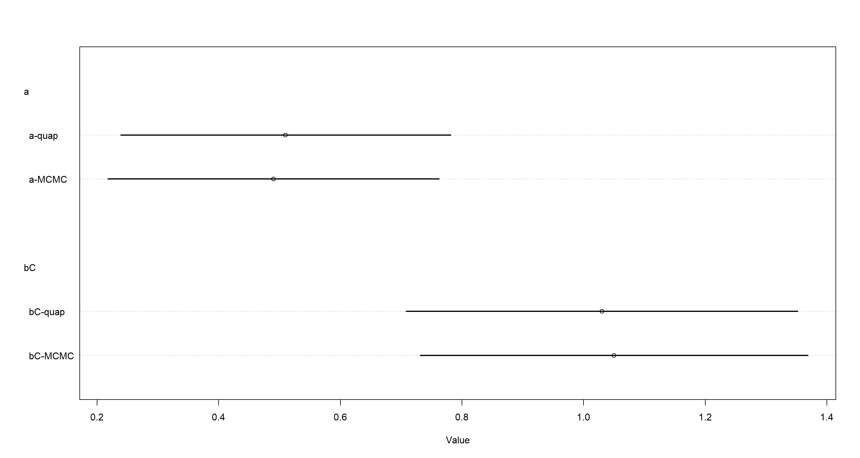
precis(m11.4, depth = 2)
##             mean        sd        5.5%       94.5%    n_eff    Rhat4
## a[1] -0.45075443 0.3331248 -0.98953991  0.06075382 698.8809 1.005361
## a[2]  3.91891754 0.8083257  2.74211339  5.24785152 901.5623 0.998913
## a[3] -0.75442240 0.3312761 -1.28541454 -0.24524706 699.9722 1.003839
## a[4] -0.76567679 0.3369675 -1.30127846 -0.23894487 857.8075 1.003696
## a[5] -0.44359742 0.3267862 -0.97201306  0.07594653 674.2582 1.005466
## a[6]  0.46443104 0.3317285 -0.05869988  0.99613901 810.7556 1.003976
## a[7]  1.96593450 0.4242551  1.31622570  2.65044970 899.8839 1.001162
## b[1] -0.03793442 0.2858597 -0.49368201  0.42539507 686.8362 1.005492
## b[2]  0.48704573 0.2866880  0.03296044  0.95020885 703.0115 1.004415
## b[3] -0.38805106 0.2815222 -0.82364579  0.06867557 639.3679 1.004886
## b[4]  0.37075102 0.2834843 -0.08070002  0.83024441 623.7355 1.006236
## Quap Model
m11.4quap <- quap(
  alist(
    pulled_left ~ dbinom(1, p),
    logit(p) <- a[actor] + b[treatment],
    a[actor] ~ dnorm(0, 1.5),
    b[treatment] ~ dnorm(0, 0.5)
  ),
  data = dat_list
)
plot(coeftab(m11.4, m11.4quap),
  labels = paste(rep(rownames(coeftab(m11.4, m11.4quap)@coefs), each = 2),
    rep(c("MCMC", "quap"), nrow(coeftab(m11.4, m11.4quap)@coefs) * 2),
    sep = "-"
  )
)
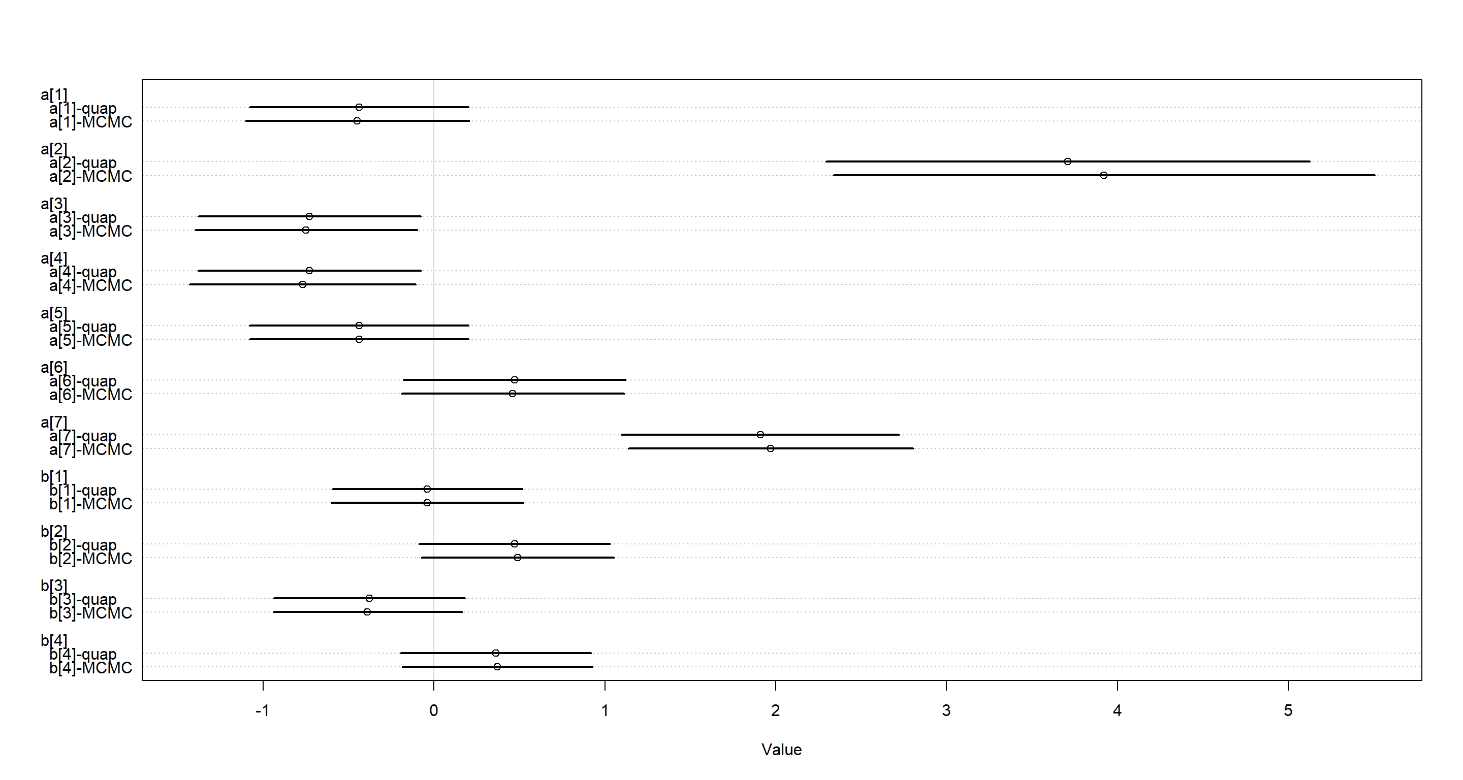
Looking at these parameter estimates, it is apparent that quadratic approximation is doing a good job in this case. The only noticeable difference lies with a[2] which shows a higher estimate with the ulam model. Let’s look at the densities of the estimates of this parameter:
post <- extract.samples(m11.4)
postq <- extract.samples(m11.4quap)
dens(post$a[, 2], lwd = 2)
dens(postq$a[, 2], add = TRUE, lwd = 2, col = rangi2)
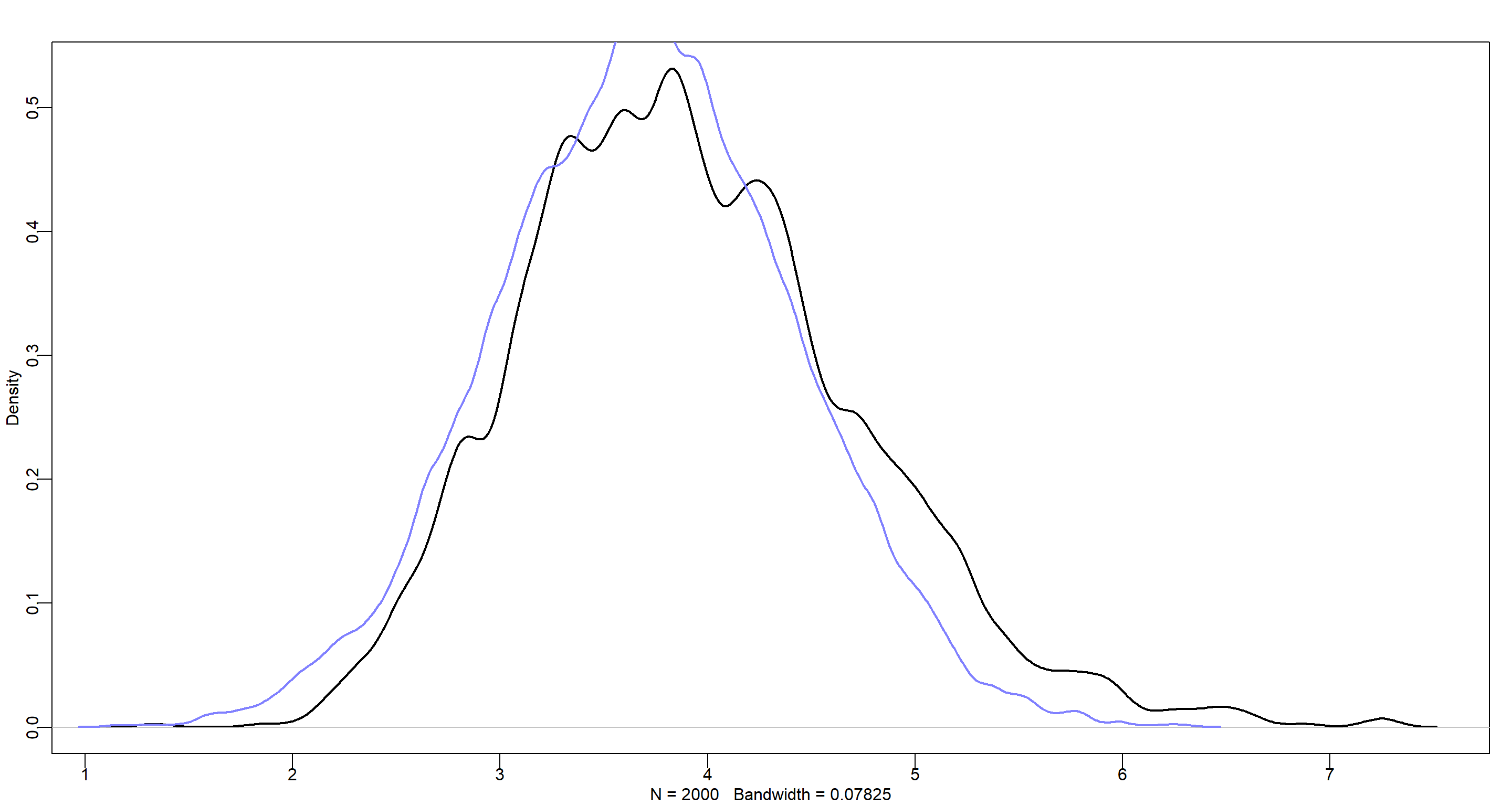
The ulam model (in black) placed more probability mass in the upper end of the tail which ends up pushing the mean of this posterior distribution further to the right when compared to that of the quadratic approximation model. This is because the quadratic approximation assumes the posterior distribution to be Gaussian thus producing a symmetric distribution with less probability mass in the upper tail.
Practice H2
Question: Use WAIC to compare the chimpanzee model that includes a unique intercept for each actor, m11.4 (page 338), to the simpler models fit in the same section.
Answer: The models in question are:
- Intercept only model:
m11.1 <- quap(
  alist(
    pulled_left ~ dbinom(1, p),
    logit(p) <- a,
    a ~ dnorm(0, 10)
  ),
  data = d
)
- Intercept and Treatment model:
m11.3 <- quap(
  alist(
    pulled_left ~ dbinom(1, p),
    logit(p) <- a + b[treatment],
    a ~ dnorm(0, 1.5),
    b[treatment] ~ dnorm(0, 0.5)
  ),
  data = d
)
- Individual Intercept and Treatment model:
m11.4 <- ulam(
  alist(
    pulled_left ~ dbinom(1, p),
    logit(p) <- a[actor] + b[treatment],
    a[actor] ~ dnorm(0, 1.5),
    b[treatment] ~ dnorm(0, 0.5)
  ),
  data = dat_list, chains = 4, log_lik = TRUE
)
##
## SAMPLING FOR MODEL '80e2b6267e3dc4ff0c2916d0cf0879e8' NOW (CHAIN 1).
## Chain 1:
## Chain 1: Gradient evaluation took 0 seconds
## Chain 1: 1000 transitions using 10 leapfrog steps per transition would take 0 seconds.
## Chain 1: Adjust your expectations accordingly!
## Chain 1:
## Chain 1:
## Chain 1: Iteration:   1 / 1000 [  0%]  (Warmup)
## Chain 1: Iteration: 100 / 1000 [ 10%]  (Warmup)
## Chain 1: Iteration: 200 / 1000 [ 20%]  (Warmup)
## Chain 1: Iteration: 300 / 1000 [ 30%]  (Warmup)
## Chain 1: Iteration: 400 / 1000 [ 40%]  (Warmup)
## Chain 1: Iteration: 500 / 1000 [ 50%]  (Warmup)
## Chain 1: Iteration: 501 / 1000 [ 50%]  (Sampling)
## Chain 1: Iteration: 600 / 1000 [ 60%]  (Sampling)
## Chain 1: Iteration: 700 / 1000 [ 70%]  (Sampling)
## Chain 1: Iteration: 800 / 1000 [ 80%]  (Sampling)
## Chain 1: Iteration: 900 / 1000 [ 90%]  (Sampling)
## Chain 1: Iteration: 1000 / 1000 [100%]  (Sampling)
## Chain 1:
## Chain 1:  Elapsed Time: 0.978 seconds (Warm-up)
## Chain 1:                0.775 seconds (Sampling)
## Chain 1:                1.753 seconds (Total)
## Chain 1:
##
## SAMPLING FOR MODEL '80e2b6267e3dc4ff0c2916d0cf0879e8' NOW (CHAIN 2).
## Chain 2:
## Chain 2: Gradient evaluation took 0 seconds
## Chain 2: 1000 transitions using 10 leapfrog steps per transition would take 0 seconds.
## Chain 2: Adjust your expectations accordingly!
## Chain 2:
## Chain 2:
## Chain 2: Iteration:   1 / 1000 [  0%]  (Warmup)
## Chain 2: Iteration: 100 / 1000 [ 10%]  (Warmup)
## Chain 2: Iteration: 200 / 1000 [ 20%]  (Warmup)
## Chain 2: Iteration: 300 / 1000 [ 30%]  (Warmup)
## Chain 2: Iteration: 400 / 1000 [ 40%]  (Warmup)
## Chain 2: Iteration: 500 / 1000 [ 50%]  (Warmup)
## Chain 2: Iteration: 501 / 1000 [ 50%]  (Sampling)
## Chain 2: Iteration: 600 / 1000 [ 60%]  (Sampling)
## Chain 2: Iteration: 700 / 1000 [ 70%]  (Sampling)
## Chain 2: Iteration: 800 / 1000 [ 80%]  (Sampling)
## Chain 2: Iteration: 900 / 1000 [ 90%]  (Sampling)
## Chain 2: Iteration: 1000 / 1000 [100%]  (Sampling)
## Chain 2:
## Chain 2:  Elapsed Time: 0.865 seconds (Warm-up)
## Chain 2:                0.834 seconds (Sampling)
## Chain 2:                1.699 seconds (Total)
## Chain 2:
##
## SAMPLING FOR MODEL '80e2b6267e3dc4ff0c2916d0cf0879e8' NOW (CHAIN 3).
## Chain 3:
## Chain 3: Gradient evaluation took 0 seconds
## Chain 3: 1000 transitions using 10 leapfrog steps per transition would take 0 seconds.
## Chain 3: Adjust your expectations accordingly!
## Chain 3:
## Chain 3:
## Chain 3: Iteration:   1 / 1000 [  0%]  (Warmup)
## Chain 3: Iteration: 100 / 1000 [ 10%]  (Warmup)
## Chain 3: Iteration: 200 / 1000 [ 20%]  (Warmup)
## Chain 3: Iteration: 300 / 1000 [ 30%]  (Warmup)
## Chain 3: Iteration: 400 / 1000 [ 40%]  (Warmup)
## Chain 3: Iteration: 500 / 1000 [ 50%]  (Warmup)
## Chain 3: Iteration: 501 / 1000 [ 50%]  (Sampling)
## Chain 3: Iteration: 600 / 1000 [ 60%]  (Sampling)
## Chain 3: Iteration: 700 / 1000 [ 70%]  (Sampling)
## Chain 3: Iteration: 800 / 1000 [ 80%]  (Sampling)
## Chain 3: Iteration: 900 / 1000 [ 90%]  (Sampling)
## Chain 3: Iteration: 1000 / 1000 [100%]  (Sampling)
## Chain 3:
## Chain 3:  Elapsed Time: 0.857 seconds (Warm-up)
## Chain 3:                0.612 seconds (Sampling)
## Chain 3:                1.469 seconds (Total)
## Chain 3:
##
## SAMPLING FOR MODEL '80e2b6267e3dc4ff0c2916d0cf0879e8' NOW (CHAIN 4).
## Chain 4:
## Chain 4: Gradient evaluation took 0 seconds
## Chain 4: 1000 transitions using 10 leapfrog steps per transition would take 0 seconds.
## Chain 4: Adjust your expectations accordingly!
## Chain 4:
## Chain 4:
## Chain 4: Iteration:   1 / 1000 [  0%]  (Warmup)
## Chain 4: Iteration: 100 / 1000 [ 10%]  (Warmup)
## Chain 4: Iteration: 200 / 1000 [ 20%]  (Warmup)
## Chain 4: Iteration: 300 / 1000 [ 30%]  (Warmup)
## Chain 4: Iteration: 400 / 1000 [ 40%]  (Warmup)
## Chain 4: Iteration: 500 / 1000 [ 50%]  (Warmup)
## Chain 4: Iteration: 501 / 1000 [ 50%]  (Sampling)
## Chain 4: Iteration: 600 / 1000 [ 60%]  (Sampling)
## Chain 4: Iteration: 700 / 1000 [ 70%]  (Sampling)
## Chain 4: Iteration: 800 / 1000 [ 80%]  (Sampling)
## Chain 4: Iteration: 900 / 1000 [ 90%]  (Sampling)
## Chain 4: Iteration: 1000 / 1000 [100%]  (Sampling)
## Chain 4:
## Chain 4:  Elapsed Time: 0.919 seconds (Warm-up)
## Chain 4:                0.937 seconds (Sampling)
## Chain 4:                1.856 seconds (Total)
## Chain 4:
To compare these, we can run:
(comp <- compare(m11.1, m11.3, m11.4))
##           WAIC        SE    dWAIC      dSE    pWAIC       weight
## m11.4 532.4794 18.927161   0.0000       NA 8.572123 1.000000e+00
## m11.3 682.4152  8.973761 149.9358 18.37892 3.553310 2.765987e-33
## m11.1 687.9540  6.994012 155.4746 18.91781 1.004840 1.734267e-34
plot(comp)
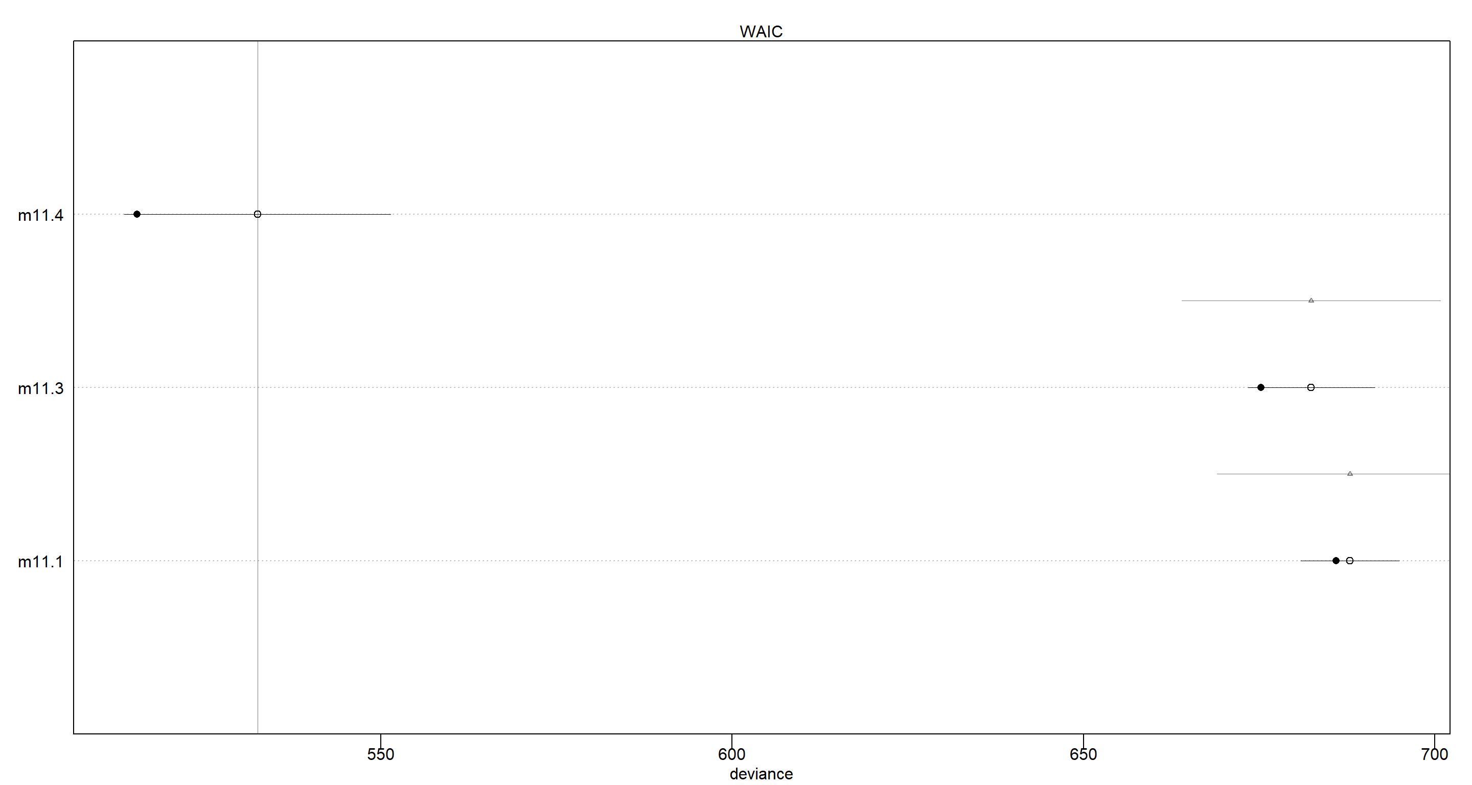
This shows clearly that the model accounting for individual intercepts as well as treatment effects (m11.4) outperforms the simpler models.
Practice H3
Question: The data contained in library(MASS);data(eagles) are records of salmon pirating attempts by Bald Eagles in Washington State. See ?eagles for details. While one eagle feeds, sometimes another will swoop in and try to steal the salmon from it. Call the feeding eagle the “victim” and the thief the “pirate.” Use the available data to build a binomial GLM of successful pirating attempts.
Answer:
library(MASS)
data(eagles)
d <- eagles
Part A
Question: Consider the following model:
$$y_i ∼ Binomial(n_i, p_i)$$ $$log\frac{p_i}{1 − p_i} = α + β_PP_i + β_VV_i + β_AA_i $$ $$α ∼ Normal(0, 1.5)$$ $$β_P ∼ Normal(0, 0.5)$$ $$β_V ∼ Normal(0, 0.5)$$ $$β_A ∼ Normal(0, 0.5)$$ where $y$ is the number of successful attempts, $n$ is the total number of attempts, $P$ is a dummy variable indicating whether or not the pirate had large body size, $V$ is a dummy variable indicating whether or not the victim had large body size, and finally $A$ is a dummy variable indicating whether or not the pirate was an adult.
Fit the model above to the eagles data, using both quap and ulam. Is the quadratic approximation okay?
Answer: First, we have to make our dummy variables:
d$pirateL <- ifelse(d$P == "L", 1, 0)
d$victimL <- ifelse(d$V == "L", 1, 0)
d$pirateA <- ifelse(d$A == "A", 1, 0)
Fitting the models is now trivial:
# define model list specification
f <- alist(
  y ~ dbinom(n, p),
  logit(p) <- a + bP * pirateL + bV * victimL + bA * pirateA,
  a ~ dnorm(0, 1.5),
  bP ~ dnorm(0, .5),
  bV ~ dnorm(0, .5),
  bA ~ dnorm(0, .5)
)
## quap model
mH3quap <- quap(f, data = d)
## ulam model
mH3ulam <- ulam(f, data = d, chains = 4, log_lik = TRUE)
##
## SAMPLING FOR MODEL '4eaf24dd51e5e9fce10e2cc7d32e0b01' NOW (CHAIN 1).
## Chain 1:
## Chain 1: Gradient evaluation took 0 seconds
## Chain 1: 1000 transitions using 10 leapfrog steps per transition would take 0 seconds.
## Chain 1: Adjust your expectations accordingly!
## Chain 1:
## Chain 1:
## Chain 1: Iteration:   1 / 1000 [  0%]  (Warmup)
## Chain 1: Iteration: 100 / 1000 [ 10%]  (Warmup)
## Chain 1: Iteration: 200 / 1000 [ 20%]  (Warmup)
## Chain 1: Iteration: 300 / 1000 [ 30%]  (Warmup)
## Chain 1: Iteration: 400 / 1000 [ 40%]  (Warmup)
## Chain 1: Iteration: 500 / 1000 [ 50%]  (Warmup)
## Chain 1: Iteration: 501 / 1000 [ 50%]  (Sampling)
## Chain 1: Iteration: 600 / 1000 [ 60%]  (Sampling)
## Chain 1: Iteration: 700 / 1000 [ 70%]  (Sampling)
## Chain 1: Iteration: 800 / 1000 [ 80%]  (Sampling)
## Chain 1: Iteration: 900 / 1000 [ 90%]  (Sampling)
## Chain 1: Iteration: 1000 / 1000 [100%]  (Sampling)
## Chain 1:
## Chain 1:  Elapsed Time: 0.07 seconds (Warm-up)
## Chain 1:                0.066 seconds (Sampling)
## Chain 1:                0.136 seconds (Total)
## Chain 1:
##
## SAMPLING FOR MODEL '4eaf24dd51e5e9fce10e2cc7d32e0b01' NOW (CHAIN 2).
## Chain 2:
## Chain 2: Gradient evaluation took 0 seconds
## Chain 2: 1000 transitions using 10 leapfrog steps per transition would take 0 seconds.
## Chain 2: Adjust your expectations accordingly!
## Chain 2:
## Chain 2:
## Chain 2: Iteration:   1 / 1000 [  0%]  (Warmup)
## Chain 2: Iteration: 100 / 1000 [ 10%]  (Warmup)
## Chain 2: Iteration: 200 / 1000 [ 20%]  (Warmup)
## Chain 2: Iteration: 300 / 1000 [ 30%]  (Warmup)
## Chain 2: Iteration: 400 / 1000 [ 40%]  (Warmup)
## Chain 2: Iteration: 500 / 1000 [ 50%]  (Warmup)
## Chain 2: Iteration: 501 / 1000 [ 50%]  (Sampling)
## Chain 2: Iteration: 600 / 1000 [ 60%]  (Sampling)
## Chain 2: Iteration: 700 / 1000 [ 70%]  (Sampling)
## Chain 2: Iteration: 800 / 1000 [ 80%]  (Sampling)
## Chain 2: Iteration: 900 / 1000 [ 90%]  (Sampling)
## Chain 2: Iteration: 1000 / 1000 [100%]  (Sampling)
## Chain 2:
## Chain 2:  Elapsed Time: 0.08 seconds (Warm-up)
## Chain 2:                0.109 seconds (Sampling)
## Chain 2:                0.189 seconds (Total)
## Chain 2:
##
## SAMPLING FOR MODEL '4eaf24dd51e5e9fce10e2cc7d32e0b01' NOW (CHAIN 3).
## Chain 3:
## Chain 3: Gradient evaluation took 0 seconds
## Chain 3: 1000 transitions using 10 leapfrog steps per transition would take 0 seconds.
## Chain 3: Adjust your expectations accordingly!
## Chain 3:
## Chain 3:
## Chain 3: Iteration:   1 / 1000 [  0%]  (Warmup)
## Chain 3: Iteration: 100 / 1000 [ 10%]  (Warmup)
## Chain 3: Iteration: 200 / 1000 [ 20%]  (Warmup)
## Chain 3: Iteration: 300 / 1000 [ 30%]  (Warmup)
## Chain 3: Iteration: 400 / 1000 [ 40%]  (Warmup)
## Chain 3: Iteration: 500 / 1000 [ 50%]  (Warmup)
## Chain 3: Iteration: 501 / 1000 [ 50%]  (Sampling)
## Chain 3: Iteration: 600 / 1000 [ 60%]  (Sampling)
## Chain 3: Iteration: 700 / 1000 [ 70%]  (Sampling)
## Chain 3: Iteration: 800 / 1000 [ 80%]  (Sampling)
## Chain 3: Iteration: 900 / 1000 [ 90%]  (Sampling)
## Chain 3: Iteration: 1000 / 1000 [100%]  (Sampling)
## Chain 3:
## Chain 3:  Elapsed Time: 0.114 seconds (Warm-up)
## Chain 3:                0.084 seconds (Sampling)
## Chain 3:                0.198 seconds (Total)
## Chain 3:
##
## SAMPLING FOR MODEL '4eaf24dd51e5e9fce10e2cc7d32e0b01' NOW (CHAIN 4).
## Chain 4:
## Chain 4: Gradient evaluation took 0 seconds
## Chain 4: 1000 transitions using 10 leapfrog steps per transition would take 0 seconds.
## Chain 4: Adjust your expectations accordingly!
## Chain 4:
## Chain 4:
## Chain 4: Iteration:   1 / 1000 [  0%]  (Warmup)
## Chain 4: Iteration: 100 / 1000 [ 10%]  (Warmup)
## Chain 4: Iteration: 200 / 1000 [ 20%]  (Warmup)
## Chain 4: Iteration: 300 / 1000 [ 30%]  (Warmup)
## Chain 4: Iteration: 400 / 1000 [ 40%]  (Warmup)
## Chain 4: Iteration: 500 / 1000 [ 50%]  (Warmup)
## Chain 4: Iteration: 501 / 1000 [ 50%]  (Sampling)
## Chain 4: Iteration: 600 / 1000 [ 60%]  (Sampling)
## Chain 4: Iteration: 700 / 1000 [ 70%]  (Sampling)
## Chain 4: Iteration: 800 / 1000 [ 80%]  (Sampling)
## Chain 4: Iteration: 900 / 1000 [ 90%]  (Sampling)
## Chain 4: Iteration: 1000 / 1000 [100%]  (Sampling)
## Chain 4:
## Chain 4:  Elapsed Time: 0.101 seconds (Warm-up)
## Chain 4:                0.098 seconds (Sampling)
## Chain 4:                0.199 seconds (Total)
## Chain 4:
Again, we visualise the parameter estimates
plot(coeftab(mH3quap, mH3ulam),
  labels = paste(rep(rownames(coeftab(mH3quap, mH3ulam)@coefs), each = 2),
    rep(c("MCMC", "quap"), nrow(coeftab(mH3quap, mH3ulam)@coefs) * 2),
    sep = "-"
  )
)
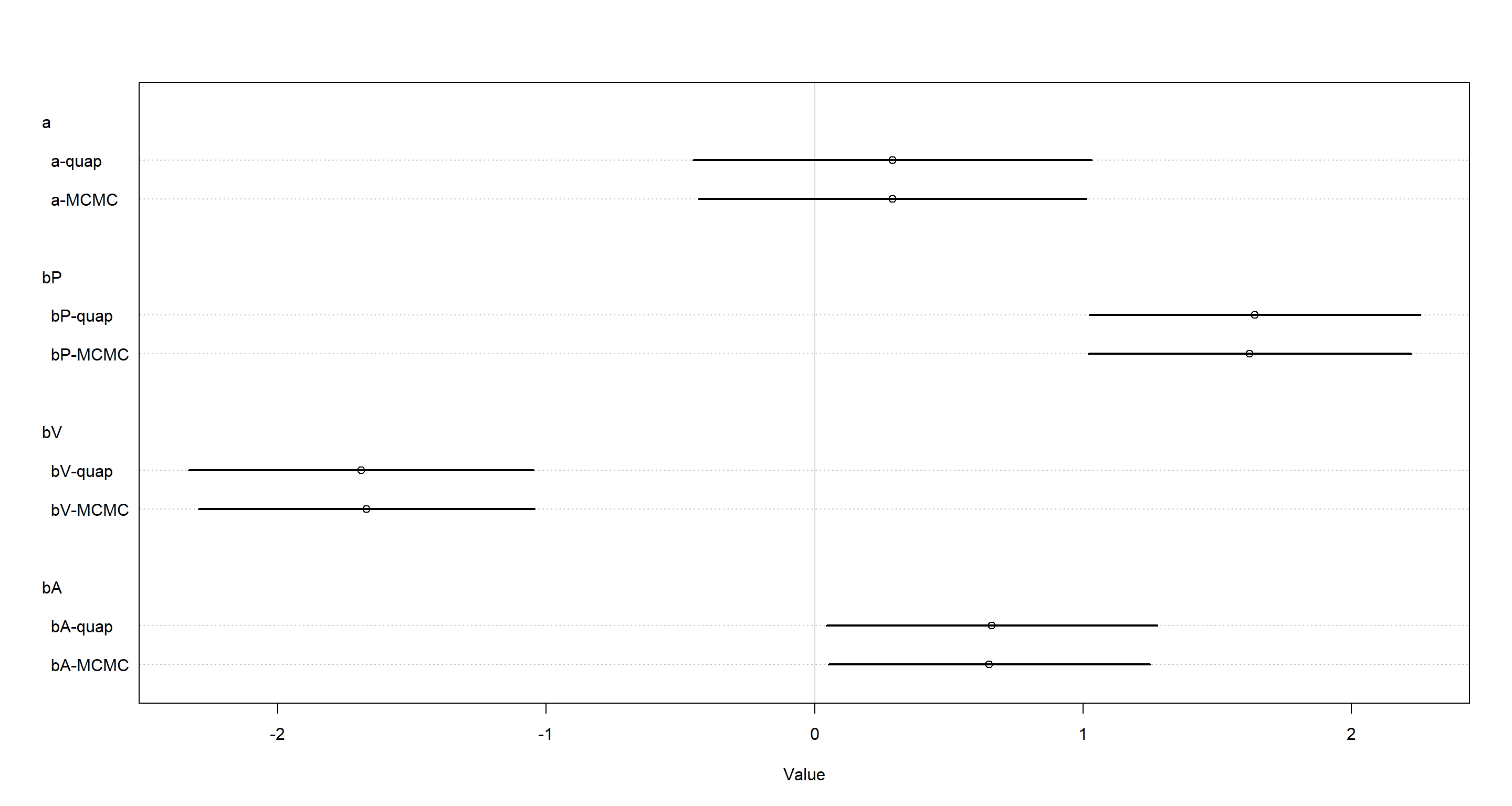
These are pretty similar looking to me.
Part B
Question: Now interpret the estimates. If the quadratic approximation turned out okay, then it’s okay
to use the quap estimates. Otherwise stick to ulam estimates. Then plot the posterior predictions. Compute and display both (1) the predicted probability of success and its 89% interval for each row ($i$) in the data, as well as (2) the predicted success count and its 89% interval. What different information does each type of posterior prediction provide?
Answer: Personally, I don’t think there’s much difference between the model estimates. Here, I am sticking to the ulam model, because I feel like it. No other reason.
Let’s start by getting a baseline understanding of how often a non-adult, small-bodied pirate is able to fetch a salmon from a small-bodied victim(all dummy variables are at value 0) - this is our intercept a. These are log-odds:
post <- extract.samples(mH3ulam)
mean(logistic(post$a))
## [1] 0.5695376
We expect about 0.57% of all of our immature, small pirates to be successful when pirating on small victims.
Now that we are armed with our baseline, we are ready to look at how our slope parameters affect what’s happening in our model.
First, we start with the effect of pirate-body-size (bP):
mean(logistic(post$a + post$bP))
## [1] 0.8678798
Damn. Large-bodied pirates win almost all of the time! We could repeat this for all slope parameters, but I find it prudent to move on to our actual task:
- Probability of success:
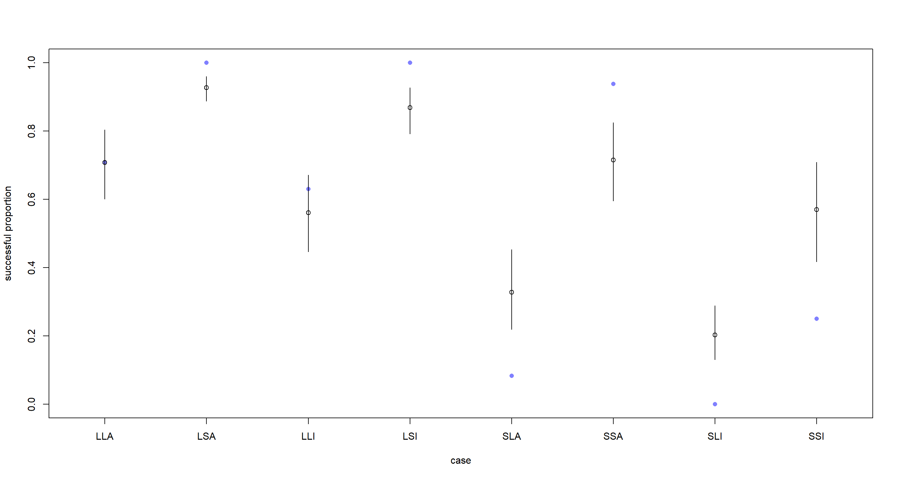
d$psuccess <- d$y / d$n # successes divided by attempts
p <- link(mH3ulam) # success probability with inverse link
## Mean and Interval Calculation
p.mean <- apply(p, 2, mean)
p.PI <- apply(p, 2, PI)
# plot raw proportions success for each case
plot(d$psuccess,
  col = rangi2,
  ylab = "successful proportion", xlab = "case", xaxt = "n",
  xlim = c(0.75, 8.25), pch = 16
)
# label cases on horizontal axis
axis(1,
  at = 1:8,
  labels = c("LLA", "LSA", "LLI", "LSI", "SLA", "SSA", "SLI", "SSI") # same order as in data frame d
)
# display posterior predicted proportions successful
points(1:8, p.mean)
for (i in 1:8) lines(c(i, i), p.PI[, i])
- Counts of successes:
y <- sim(mH3ulam) # simulate posterior for counts of successes
## Mean and Interval Calculation
y.mean <- apply(y, 2, mean)
y.PI <- apply(y, 2, PI)
# plot raw counts success for each case
plot(d$y,
  col = rangi2,
  ylab = "successful attempts", xlab = "case", xaxt = "n",
  xlim = c(0.75, 8.25), pch = 16
)
# label cases on horizontal axis
axis(1,
  at = 1:8,
  labels = c("LAL", "LAS", "LIL", "LIS", "SAL", "SAS", "SIL", "SIS")
)
# display posterior predicted successes
points(1:8, y.mean)
for (i in 1:8) lines(c(i, i), y.PI[, i])
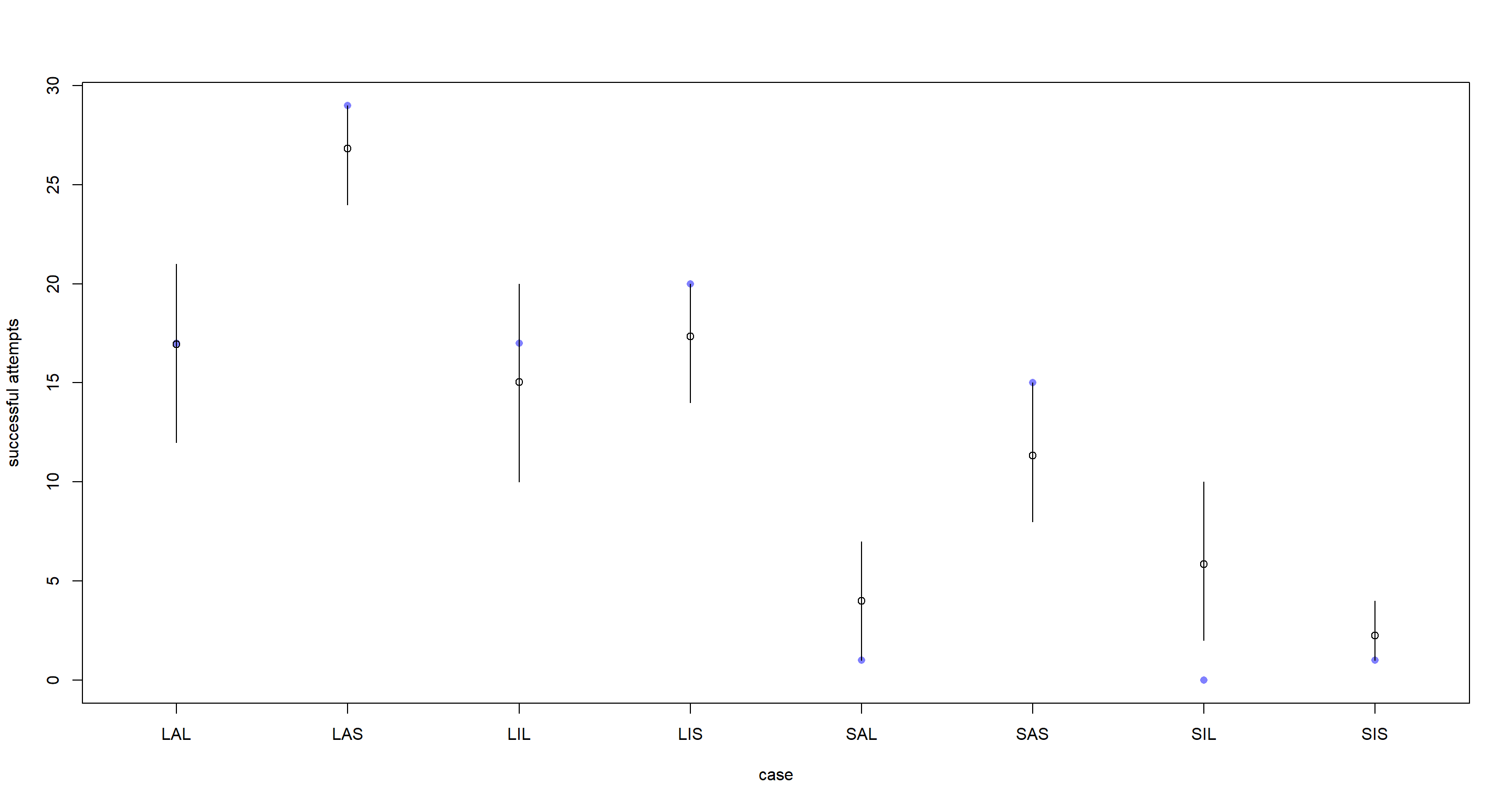
In conclusion, the probability plot makes the different settings of predictor variables more comparable because the number of piracy attempts are ignored in setting the y-axis. The count plot, however, shows the additional uncertainty stemming from the underlying sample size.
Part C
Question: Now try to improve the model. Consider an interaction between the pirate’s size and age(immature or adult). Compare this model to the previous one, using WAIC. Interpret.
Answer: Let’s fit a model with ulam containing the interaction effect we were asked for:
mH3c <- ulam(
  alist(
    y ~ dbinom(n, p),
    logit(p) <- a + bP * pirateL + bV * victimL + bA * pirateA + bPA * pirateL * pirateA,
    a ~ dnorm(0, 1.5),
    bP ~ dnorm(0, .5),
    bV ~ dnorm(0, .5),
    bA ~ dnorm(0, .5),
    bPA ~ dnorm(0, .5)
  ),
  data = d, chains = 4, log_lik = TRUE
)
##
## SAMPLING FOR MODEL '3f6607198507ea4881438baca721629d' NOW (CHAIN 1).
## Chain 1:
## Chain 1: Gradient evaluation took 0 seconds
## Chain 1: 1000 transitions using 10 leapfrog steps per transition would take 0 seconds.
## Chain 1: Adjust your expectations accordingly!
## Chain 1:
## Chain 1:
## Chain 1: Iteration:   1 / 1000 [  0%]  (Warmup)
## Chain 1: Iteration: 100 / 1000 [ 10%]  (Warmup)
## Chain 1: Iteration: 200 / 1000 [ 20%]  (Warmup)
## Chain 1: Iteration: 300 / 1000 [ 30%]  (Warmup)
## Chain 1: Iteration: 400 / 1000 [ 40%]  (Warmup)
## Chain 1: Iteration: 500 / 1000 [ 50%]  (Warmup)
## Chain 1: Iteration: 501 / 1000 [ 50%]  (Sampling)
## Chain 1: Iteration: 600 / 1000 [ 60%]  (Sampling)
## Chain 1: Iteration: 700 / 1000 [ 70%]  (Sampling)
## Chain 1: Iteration: 800 / 1000 [ 80%]  (Sampling)
## Chain 1: Iteration: 900 / 1000 [ 90%]  (Sampling)
## Chain 1: Iteration: 1000 / 1000 [100%]  (Sampling)
## Chain 1:
## Chain 1:  Elapsed Time: 0.162 seconds (Warm-up)
## Chain 1:                0.118 seconds (Sampling)
## Chain 1:                0.28 seconds (Total)
## Chain 1:
##
## SAMPLING FOR MODEL '3f6607198507ea4881438baca721629d' NOW (CHAIN 2).
## Chain 2:
## Chain 2: Gradient evaluation took 0 seconds
## Chain 2: 1000 transitions using 10 leapfrog steps per transition would take 0 seconds.
## Chain 2: Adjust your expectations accordingly!
## Chain 2:
## Chain 2:
## Chain 2: Iteration:   1 / 1000 [  0%]  (Warmup)
## Chain 2: Iteration: 100 / 1000 [ 10%]  (Warmup)
## Chain 2: Iteration: 200 / 1000 [ 20%]  (Warmup)
## Chain 2: Iteration: 300 / 1000 [ 30%]  (Warmup)
## Chain 2: Iteration: 400 / 1000 [ 40%]  (Warmup)
## Chain 2: Iteration: 500 / 1000 [ 50%]  (Warmup)
## Chain 2: Iteration: 501 / 1000 [ 50%]  (Sampling)
## Chain 2: Iteration: 600 / 1000 [ 60%]  (Sampling)
## Chain 2: Iteration: 700 / 1000 [ 70%]  (Sampling)
## Chain 2: Iteration: 800 / 1000 [ 80%]  (Sampling)
## Chain 2: Iteration: 900 / 1000 [ 90%]  (Sampling)
## Chain 2: Iteration: 1000 / 1000 [100%]  (Sampling)
## Chain 2:
## Chain 2:  Elapsed Time: 0.142 seconds (Warm-up)
## Chain 2:                0.124 seconds (Sampling)
## Chain 2:                0.266 seconds (Total)
## Chain 2:
##
## SAMPLING FOR MODEL '3f6607198507ea4881438baca721629d' NOW (CHAIN 3).
## Chain 3:
## Chain 3: Gradient evaluation took 0 seconds
## Chain 3: 1000 transitions using 10 leapfrog steps per transition would take 0 seconds.
## Chain 3: Adjust your expectations accordingly!
## Chain 3:
## Chain 3:
## Chain 3: Iteration:   1 / 1000 [  0%]  (Warmup)
## Chain 3: Iteration: 100 / 1000 [ 10%]  (Warmup)
## Chain 3: Iteration: 200 / 1000 [ 20%]  (Warmup)
## Chain 3: Iteration: 300 / 1000 [ 30%]  (Warmup)
## Chain 3: Iteration: 400 / 1000 [ 40%]  (Warmup)
## Chain 3: Iteration: 500 / 1000 [ 50%]  (Warmup)
## Chain 3: Iteration: 501 / 1000 [ 50%]  (Sampling)
## Chain 3: Iteration: 600 / 1000 [ 60%]  (Sampling)
## Chain 3: Iteration: 700 / 1000 [ 70%]  (Sampling)
## Chain 3: Iteration: 800 / 1000 [ 80%]  (Sampling)
## Chain 3: Iteration: 900 / 1000 [ 90%]  (Sampling)
## Chain 3: Iteration: 1000 / 1000 [100%]  (Sampling)
## Chain 3:
## Chain 3:  Elapsed Time: 0.141 seconds (Warm-up)
## Chain 3:                0.119 seconds (Sampling)
## Chain 3:                0.26 seconds (Total)
## Chain 3:
##
## SAMPLING FOR MODEL '3f6607198507ea4881438baca721629d' NOW (CHAIN 4).
## Chain 4:
## Chain 4: Gradient evaluation took 0 seconds
## Chain 4: 1000 transitions using 10 leapfrog steps per transition would take 0 seconds.
## Chain 4: Adjust your expectations accordingly!
## Chain 4:
## Chain 4:
## Chain 4: Iteration:   1 / 1000 [  0%]  (Warmup)
## Chain 4: Iteration: 100 / 1000 [ 10%]  (Warmup)
## Chain 4: Iteration: 200 / 1000 [ 20%]  (Warmup)
## Chain 4: Iteration: 300 / 1000 [ 30%]  (Warmup)
## Chain 4: Iteration: 400 / 1000 [ 40%]  (Warmup)
## Chain 4: Iteration: 500 / 1000 [ 50%]  (Warmup)
## Chain 4: Iteration: 501 / 1000 [ 50%]  (Sampling)
## Chain 4: Iteration: 600 / 1000 [ 60%]  (Sampling)
## Chain 4: Iteration: 700 / 1000 [ 70%]  (Sampling)
## Chain 4: Iteration: 800 / 1000 [ 80%]  (Sampling)
## Chain 4: Iteration: 900 / 1000 [ 90%]  (Sampling)
## Chain 4: Iteration: 1000 / 1000 [100%]  (Sampling)
## Chain 4:
## Chain 4:  Elapsed Time: 0.107 seconds (Warm-up)
## Chain 4:                0.12 seconds (Sampling)
## Chain 4:                0.227 seconds (Total)
## Chain 4:
compare(mH3ulam, mH3c)
##             WAIC       SE    dWAIC      dSE    pWAIC    weight
## mH3ulam 59.09875 11.34469 0.000000       NA 8.303613 0.6932173
## mH3c    60.72916 11.90457 1.630407 1.467142 9.165510 0.3067827
This is quite obviously a tie. So what about the model estimates?
plot(coeftab(mH3ulam, mH3c),
  labels = paste(rep(rownames(coeftab(mH3ulam, mH3c)@coefs), each = 2),
    rep(c("Base", "Interac"), nrow(coeftab(mH3ulam, mH3c)@coefs) * 2),
    sep = "-"
  )
)
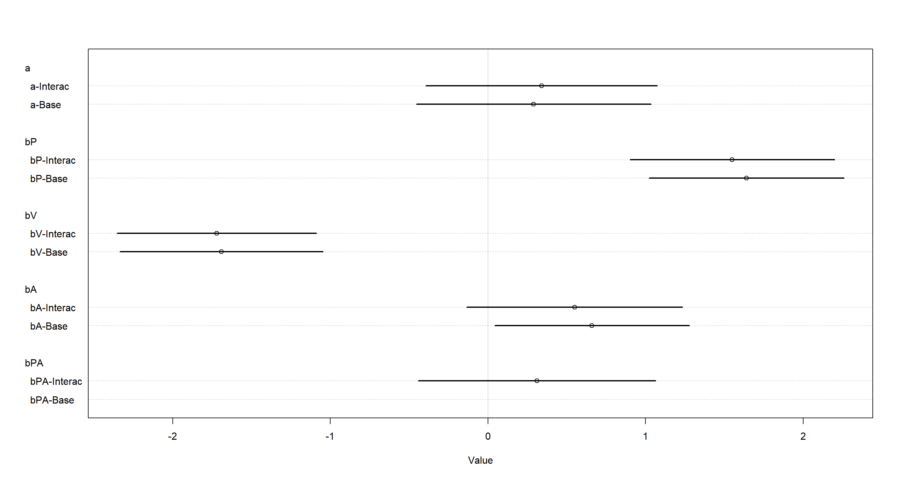 Jup, there’s not really much of a difference here. For the interaction model: the log-odds of successful piracy is just weakly bigger when the pirating individual is large and an adult. That is counter-intuitive, isn’t it? It is worth pointing out that the individual parameters for these conditions show the expected effects and the identified negative effect of their interaction may be down to the sparsity of the underlying data and we are also highly uncertain of it’s sign to begin with.
Practice H4
Question: The data contained in data(salamanders) are counts of salamanders (Plethodon elongatus) from 47 different 49$m^2$ plots in northern California. The column SALAMAN is the count in each plot, and the columns PCTCOVER and FORESTAGE are percent of ground cover and age of trees in the plot, respectively. You will model SALAMAN as a Poisson variable.
Part A
Question: Model the relationship between density and percent cover, using a log-link (same as the ex-
ample in the book and lecture). Use weakly informative priors of your choosing. Check the quadratic approximation again, by comparing quap to ulam. Then plot the expected counts and their 89% interval against percent cover. In which ways does the model do a good job? In which ways does it do a bad job?
Answer: First, we load the data and standardise the predictors to get around their inconvenient scales which do not overlap well with each other:
data(salamanders)
d <- salamanders
d$C <- standardize(d$PCTCOVER)
d$A <- standardize(d$FORESTAGE)
Now it is time to write our Poisson model:
f <- alist(
  SALAMAN ~ dpois(lambda),
  log(lambda) <- a + bC * C,
  a ~ dnorm(0, 1),
  bC ~ dnorm(0, 1)
)
That was easy enough, but do those priors make sense? Let’s simulate:
N <- 50 # 50 samples from prior
a <- rnorm(N, 0, 1)
bC <- rnorm(N, 0, 1)
C_seq <- seq(from = -2, to = 2, length.out = 30)
plot(NULL,
  xlim = c(-2, 2), ylim = c(0, 20),
  xlab = "cover(stanardized)", ylab = "salamanders"
)
for (i in 1:N) {
  lines(C_seq, exp(a[i] + bC[i] * C_seq), col = grau(), lwd = 1.5)
}
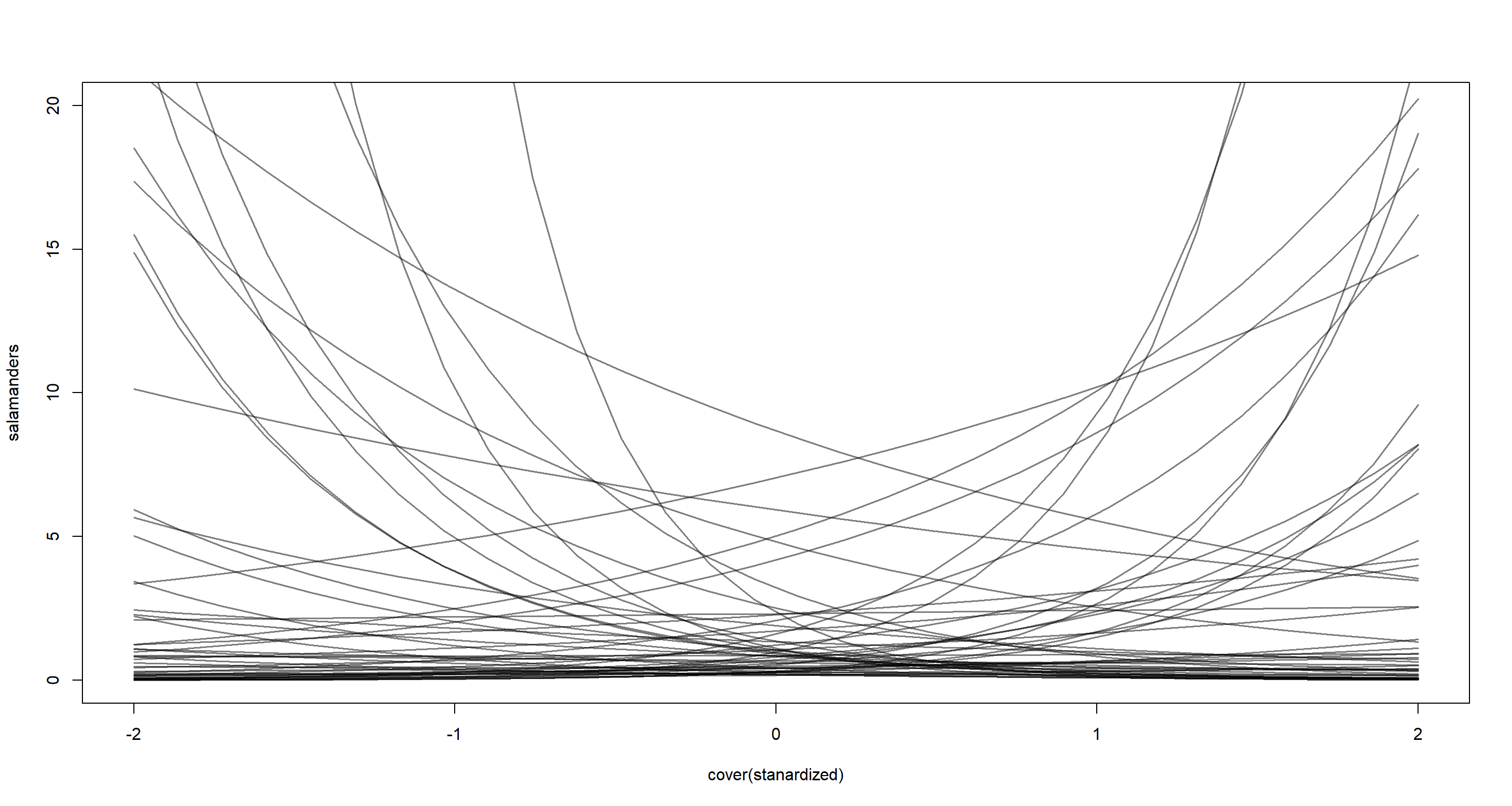
While not terrible (the prior allows your some explosive trends, but mostly sticks to a reasonable count of individuals), we may want to consider making the prior a bit more informative:
bC <- rnorm(N, 0, 0.5)
plot(NULL,
  xlim = c(-2, 2), ylim = c(0, 20),
  xlab = "cover(stanardized)", ylab = "salamanders"
)
for (i in 1:N) {
  lines(C_seq, exp(a[i] + bC[i] * C_seq), col = grau(), lwd = 1.5)
}
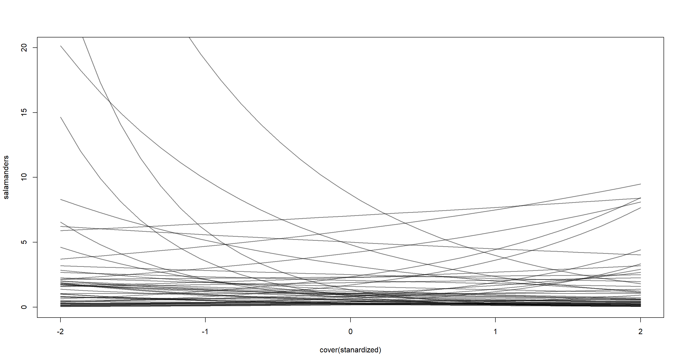 Yup - I am happy with that.
Let’s update the model specification and run it:
f <- alist(
  SALAMAN ~ dpois(lambda),
  log(lambda) <- a + bC * C,
  a ~ dnorm(0, 1),
  bC ~ dnorm(0, 0.5)
)
mH4a <- ulam(f, data = d, chains = 4)
##
## SAMPLING FOR MODEL 'ce27f50b1ba56f91eaeb68bb1bf4432c' NOW (CHAIN 1).
## Chain 1:
## Chain 1: Gradient evaluation took 0 seconds
## Chain 1: 1000 transitions using 10 leapfrog steps per transition would take 0 seconds.
## Chain 1: Adjust your expectations accordingly!
## Chain 1:
## Chain 1:
## Chain 1: Iteration:   1 / 1000 [  0%]  (Warmup)
## Chain 1: Iteration: 100 / 1000 [ 10%]  (Warmup)
## Chain 1: Iteration: 200 / 1000 [ 20%]  (Warmup)
## Chain 1: Iteration: 300 / 1000 [ 30%]  (Warmup)
## Chain 1: Iteration: 400 / 1000 [ 40%]  (Warmup)
## Chain 1: Iteration: 500 / 1000 [ 50%]  (Warmup)
## Chain 1: Iteration: 501 / 1000 [ 50%]  (Sampling)
## Chain 1: Iteration: 600 / 1000 [ 60%]  (Sampling)
## Chain 1: Iteration: 700 / 1000 [ 70%]  (Sampling)
## Chain 1: Iteration: 800 / 1000 [ 80%]  (Sampling)
## Chain 1: Iteration: 900 / 1000 [ 90%]  (Sampling)
## Chain 1: Iteration: 1000 / 1000 [100%]  (Sampling)
## Chain 1:
## Chain 1:  Elapsed Time: 0.045 seconds (Warm-up)
## Chain 1:                0.046 seconds (Sampling)
## Chain 1:                0.091 seconds (Total)
## Chain 1:
##
## SAMPLING FOR MODEL 'ce27f50b1ba56f91eaeb68bb1bf4432c' NOW (CHAIN 2).
## Chain 2:
## Chain 2: Gradient evaluation took 0 seconds
## Chain 2: 1000 transitions using 10 leapfrog steps per transition would take 0 seconds.
## Chain 2: Adjust your expectations accordingly!
## Chain 2:
## Chain 2:
## Chain 2: Iteration:   1 / 1000 [  0%]  (Warmup)
## Chain 2: Iteration: 100 / 1000 [ 10%]  (Warmup)
## Chain 2: Iteration: 200 / 1000 [ 20%]  (Warmup)
## Chain 2: Iteration: 300 / 1000 [ 30%]  (Warmup)
## Chain 2: Iteration: 400 / 1000 [ 40%]  (Warmup)
## Chain 2: Iteration: 500 / 1000 [ 50%]  (Warmup)
## Chain 2: Iteration: 501 / 1000 [ 50%]  (Sampling)
## Chain 2: Iteration: 600 / 1000 [ 60%]  (Sampling)
## Chain 2: Iteration: 700 / 1000 [ 70%]  (Sampling)
## Chain 2: Iteration: 800 / 1000 [ 80%]  (Sampling)
## Chain 2: Iteration: 900 / 1000 [ 90%]  (Sampling)
## Chain 2: Iteration: 1000 / 1000 [100%]  (Sampling)
## Chain 2:
## Chain 2:  Elapsed Time: 0.054 seconds (Warm-up)
## Chain 2:                0.062 seconds (Sampling)
## Chain 2:                0.116 seconds (Total)
## Chain 2:
##
## SAMPLING FOR MODEL 'ce27f50b1ba56f91eaeb68bb1bf4432c' NOW (CHAIN 3).
## Chain 3:
## Chain 3: Gradient evaluation took 0 seconds
## Chain 3: 1000 transitions using 10 leapfrog steps per transition would take 0 seconds.
## Chain 3: Adjust your expectations accordingly!
## Chain 3:
## Chain 3:
## Chain 3: Iteration:   1 / 1000 [  0%]  (Warmup)
## Chain 3: Iteration: 100 / 1000 [ 10%]  (Warmup)
## Chain 3: Iteration: 200 / 1000 [ 20%]  (Warmup)
## Chain 3: Iteration: 300 / 1000 [ 30%]  (Warmup)
## Chain 3: Iteration: 400 / 1000 [ 40%]  (Warmup)
## Chain 3: Iteration: 500 / 1000 [ 50%]  (Warmup)
## Chain 3: Iteration: 501 / 1000 [ 50%]  (Sampling)
## Chain 3: Iteration: 600 / 1000 [ 60%]  (Sampling)
## Chain 3: Iteration: 700 / 1000 [ 70%]  (Sampling)
## Chain 3: Iteration: 800 / 1000 [ 80%]  (Sampling)
## Chain 3: Iteration: 900 / 1000 [ 90%]  (Sampling)
## Chain 3: Iteration: 1000 / 1000 [100%]  (Sampling)
## Chain 3:
## Chain 3:  Elapsed Time: 0.052 seconds (Warm-up)
## Chain 3:                0.051 seconds (Sampling)
## Chain 3:                0.103 seconds (Total)
## Chain 3:
##
## SAMPLING FOR MODEL 'ce27f50b1ba56f91eaeb68bb1bf4432c' NOW (CHAIN 4).
## Chain 4:
## Chain 4: Gradient evaluation took 0 seconds
## Chain 4: 1000 transitions using 10 leapfrog steps per transition would take 0 seconds.
## Chain 4: Adjust your expectations accordingly!
## Chain 4:
## Chain 4:
## Chain 4: Iteration:   1 / 1000 [  0%]  (Warmup)
## Chain 4: Iteration: 100 / 1000 [ 10%]  (Warmup)
## Chain 4: Iteration: 200 / 1000 [ 20%]  (Warmup)
## Chain 4: Iteration: 300 / 1000 [ 30%]  (Warmup)
## Chain 4: Iteration: 400 / 1000 [ 40%]  (Warmup)
## Chain 4: Iteration: 500 / 1000 [ 50%]  (Warmup)
## Chain 4: Iteration: 501 / 1000 [ 50%]  (Sampling)
## Chain 4: Iteration: 600 / 1000 [ 60%]  (Sampling)
## Chain 4: Iteration: 700 / 1000 [ 70%]  (Sampling)
## Chain 4: Iteration: 800 / 1000 [ 80%]  (Sampling)
## Chain 4: Iteration: 900 / 1000 [ 90%]  (Sampling)
## Chain 4: Iteration: 1000 / 1000 [100%]  (Sampling)
## Chain 4:
## Chain 4:  Elapsed Time: 0.065 seconds (Warm-up)
## Chain 4:                0.058 seconds (Sampling)
## Chain 4:                0.123 seconds (Total)
## Chain 4:
mH4aquap <- quap(f, data = d)
plot(coeftab(mH4a, mH4aquap),
  labels = paste(rep(rownames(coeftab(mH4a, mH4aquap)@coefs), each = 2),
    rep(c("MCMC", "quap"), nrow(coeftab(mH4a, mH4aquap)@coefs) * 2),
    sep = "-"
  )
)
 Again, both models are doing fine and we continue to our plotting of expected counts and their interval with the
 ulam model:
plot(d$C, d$SALAMAN,
  col = rangi2, lwd = 2,
  xlab = "cover(standardized)", ylab = "salamanders observed"
)
C_seq <- seq(from = -2, to = 2, length.out = 30)
l <- link(mH4a, data = list(C = C_seq))
lines(C_seq, colMeans(l))
shade(apply(l, 2, PI), C_seq)
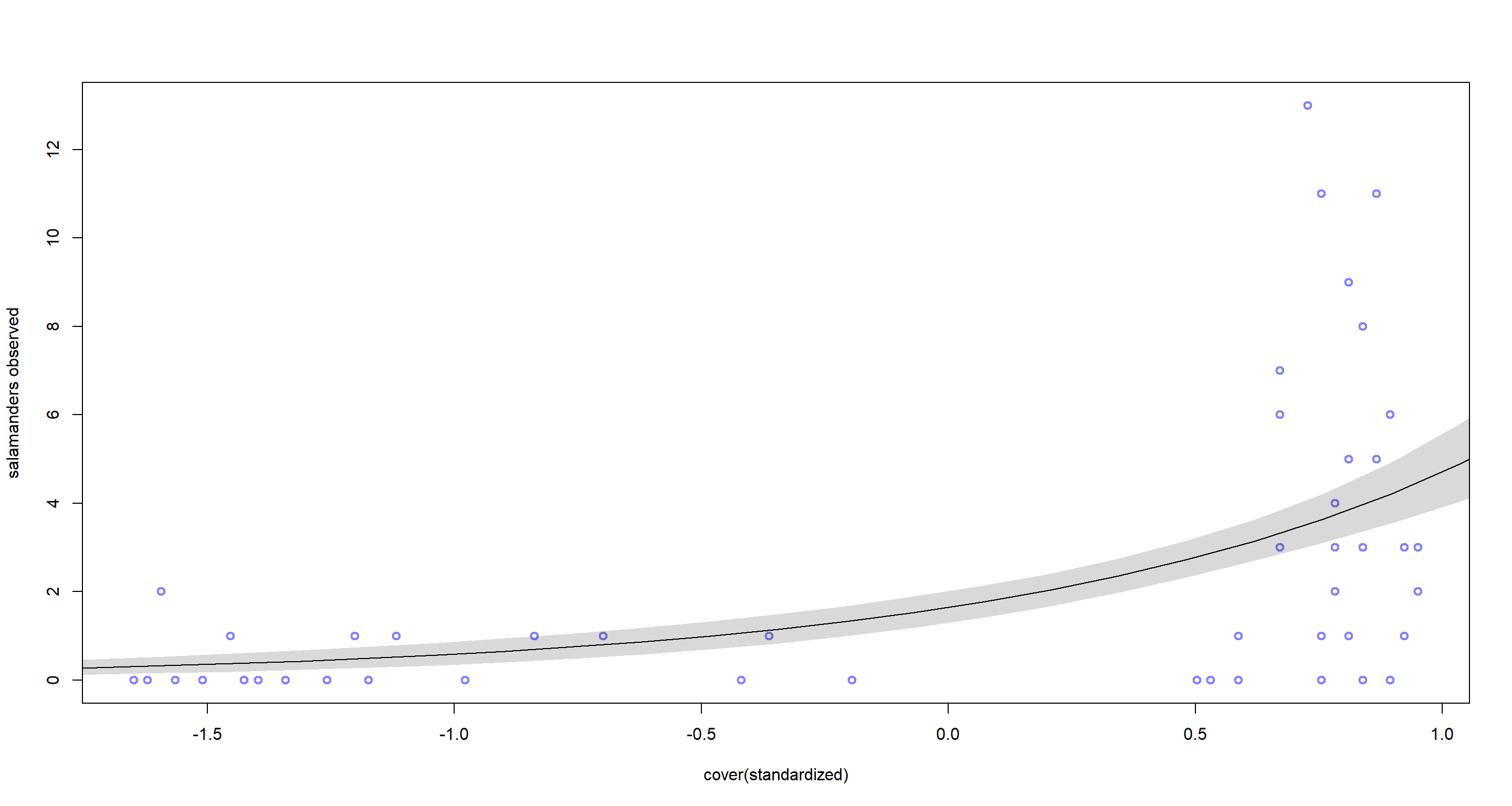 Well that model doesn’t fit all that nicely and the data seems over-dispersed to me.
Part B
Question: Can you improve the model by using the other predictor, FORESTAGE? Try any models you think useful. Can you explain why FORESTAGE helps or does not help with prediction?
Answer: Forest cover might be confounded by forest age. The older a forest, the bigger its coverage? A model to investigate this could look like this:
f2 <- alist(
  SALAMAN ~ dpois(lambda),
  log(lambda) <- a + bC * C + bA * A,
  a ~ dnorm(0, 1),
  c(bC, bA) ~ dnorm(0, 0.5)
)
mH4b <- ulam(f2, data = d, chains = 4)
##
## SAMPLING FOR MODEL '4850e2c86bda45f77f837aaee26a4da5' NOW (CHAIN 1).
## Chain 1:
## Chain 1: Gradient evaluation took 0 seconds
## Chain 1: 1000 transitions using 10 leapfrog steps per transition would take 0 seconds.
## Chain 1: Adjust your expectations accordingly!
## Chain 1:
## Chain 1:
## Chain 1: Iteration:   1 / 1000 [  0%]  (Warmup)
## Chain 1: Iteration: 100 / 1000 [ 10%]  (Warmup)
## Chain 1: Iteration: 200 / 1000 [ 20%]  (Warmup)
## Chain 1: Iteration: 300 / 1000 [ 30%]  (Warmup)
## Chain 1: Iteration: 400 / 1000 [ 40%]  (Warmup)
## Chain 1: Iteration: 500 / 1000 [ 50%]  (Warmup)
## Chain 1: Iteration: 501 / 1000 [ 50%]  (Sampling)
## Chain 1: Iteration: 600 / 1000 [ 60%]  (Sampling)
## Chain 1: Iteration: 700 / 1000 [ 70%]  (Sampling)
## Chain 1: Iteration: 800 / 1000 [ 80%]  (Sampling)
## Chain 1: Iteration: 900 / 1000 [ 90%]  (Sampling)
## Chain 1: Iteration: 1000 / 1000 [100%]  (Sampling)
## Chain 1:
## Chain 1:  Elapsed Time: 0.066 seconds (Warm-up)
## Chain 1:                0.067 seconds (Sampling)
## Chain 1:                0.133 seconds (Total)
## Chain 1:
##
## SAMPLING FOR MODEL '4850e2c86bda45f77f837aaee26a4da5' NOW (CHAIN 2).
## Chain 2:
## Chain 2: Gradient evaluation took 0 seconds
## Chain 2: 1000 transitions using 10 leapfrog steps per transition would take 0 seconds.
## Chain 2: Adjust your expectations accordingly!
## Chain 2:
## Chain 2:
## Chain 2: Iteration:   1 / 1000 [  0%]  (Warmup)
## Chain 2: Iteration: 100 / 1000 [ 10%]  (Warmup)
## Chain 2: Iteration: 200 / 1000 [ 20%]  (Warmup)
## Chain 2: Iteration: 300 / 1000 [ 30%]  (Warmup)
## Chain 2: Iteration: 400 / 1000 [ 40%]  (Warmup)
## Chain 2: Iteration: 500 / 1000 [ 50%]  (Warmup)
## Chain 2: Iteration: 501 / 1000 [ 50%]  (Sampling)
## Chain 2: Iteration: 600 / 1000 [ 60%]  (Sampling)
## Chain 2: Iteration: 700 / 1000 [ 70%]  (Sampling)
## Chain 2: Iteration: 800 / 1000 [ 80%]  (Sampling)
## Chain 2: Iteration: 900 / 1000 [ 90%]  (Sampling)
## Chain 2: Iteration: 1000 / 1000 [100%]  (Sampling)
## Chain 2:
## Chain 2:  Elapsed Time: 0.068 seconds (Warm-up)
## Chain 2:                0.079 seconds (Sampling)
## Chain 2:                0.147 seconds (Total)
## Chain 2:
##
## SAMPLING FOR MODEL '4850e2c86bda45f77f837aaee26a4da5' NOW (CHAIN 3).
## Chain 3:
## Chain 3: Gradient evaluation took 0 seconds
## Chain 3: 1000 transitions using 10 leapfrog steps per transition would take 0 seconds.
## Chain 3: Adjust your expectations accordingly!
## Chain 3:
## Chain 3:
## Chain 3: Iteration:   1 / 1000 [  0%]  (Warmup)
## Chain 3: Iteration: 100 / 1000 [ 10%]  (Warmup)
## Chain 3: Iteration: 200 / 1000 [ 20%]  (Warmup)
## Chain 3: Iteration: 300 / 1000 [ 30%]  (Warmup)
## Chain 3: Iteration: 400 / 1000 [ 40%]  (Warmup)
## Chain 3: Iteration: 500 / 1000 [ 50%]  (Warmup)
## Chain 3: Iteration: 501 / 1000 [ 50%]  (Sampling)
## Chain 3: Iteration: 600 / 1000 [ 60%]  (Sampling)
## Chain 3: Iteration: 700 / 1000 [ 70%]  (Sampling)
## Chain 3: Iteration: 800 / 1000 [ 80%]  (Sampling)
## Chain 3: Iteration: 900 / 1000 [ 90%]  (Sampling)
## Chain 3: Iteration: 1000 / 1000 [100%]  (Sampling)
## Chain 3:
## Chain 3:  Elapsed Time: 0.064 seconds (Warm-up)
## Chain 3:                0.062 seconds (Sampling)
## Chain 3:                0.126 seconds (Total)
## Chain 3:
##
## SAMPLING FOR MODEL '4850e2c86bda45f77f837aaee26a4da5' NOW (CHAIN 4).
## Chain 4:
## Chain 4: Gradient evaluation took 0 seconds
## Chain 4: 1000 transitions using 10 leapfrog steps per transition would take 0 seconds.
## Chain 4: Adjust your expectations accordingly!
## Chain 4:
## Chain 4:
## Chain 4: Iteration:   1 / 1000 [  0%]  (Warmup)
## Chain 4: Iteration: 100 / 1000 [ 10%]  (Warmup)
## Chain 4: Iteration: 200 / 1000 [ 20%]  (Warmup)
## Chain 4: Iteration: 300 / 1000 [ 30%]  (Warmup)
## Chain 4: Iteration: 400 / 1000 [ 40%]  (Warmup)
## Chain 4: Iteration: 500 / 1000 [ 50%]  (Warmup)
## Chain 4: Iteration: 501 / 1000 [ 50%]  (Sampling)
## Chain 4: Iteration: 600 / 1000 [ 60%]  (Sampling)
## Chain 4: Iteration: 700 / 1000 [ 70%]  (Sampling)
## Chain 4: Iteration: 800 / 1000 [ 80%]  (Sampling)
## Chain 4: Iteration: 900 / 1000 [ 90%]  (Sampling)
## Chain 4: Iteration: 1000 / 1000 [100%]  (Sampling)
## Chain 4:
## Chain 4:  Elapsed Time: 0.076 seconds (Warm-up)
## Chain 4:                0.058 seconds (Sampling)
## Chain 4:                0.134 seconds (Total)
## Chain 4:
precis(mH4b)
##          mean         sd       5.5%     94.5%     n_eff    Rhat4
## a  0.48361398 0.13609701  0.2618982 0.6896444  873.3384 1.003115
## bA 0.01904618 0.09647959 -0.1361230 0.1679860 1102.3547 1.002465
## bC 1.04260846 0.17335950  0.7795899 1.3262340  919.5342 1.000832
Fascinating! The estimate for bA is nearly $0$ with a lot of certainty (i.e. a small interval) behind it. While conditioning on percent cover, forest age does not influence salamander count. This looks like a post-treatment effect to me.
Session Info
sessionInfo()
## R version 4.0.5 (2021-03-31)
## Platform: x86_64-w64-mingw32/x64 (64-bit)
## Running under: Windows 10 x64 (build 19043)
##
## Matrix products: default
##
## locale:
## [1] LC_COLLATE=English_United Kingdom.1252  LC_CTYPE=English_United Kingdom.1252    LC_MONETARY=English_United Kingdom.1252 LC_NUMERIC=C
## [5] LC_TIME=English_United Kingdom.1252
##
## attached base packages:
## [1] parallel  stats     graphics  grDevices utils     datasets  methods   base
##
## other attached packages:
## [1] MASS_7.3-53.1        tidybayes_2.3.1      rethinking_2.13      rstan_2.21.2         ggplot2_3.3.6        StanHeaders_2.21.0-7
##
## loaded via a namespace (and not attached):
##  [1] Rcpp_1.0.7           mvtnorm_1.1-1        lattice_0.20-41      tidyr_1.1.3          prettyunits_1.1.1    ps_1.6.0             assertthat_0.2.1     digest_0.6.27        utf8_1.2.1
## [10] V8_3.4.1             plyr_1.8.6           R6_2.5.0             backports_1.2.1      stats4_4.0.5         evaluate_0.14        coda_0.19-4          highr_0.9            blogdown_1.3
## [19] pillar_1.6.0         rlang_0.4.11         curl_4.3.2           callr_3.7.0          jquerylib_0.1.4      R.utils_2.10.1       R.oo_1.24.0          rmarkdown_2.7        styler_1.4.1
## [28] stringr_1.4.0        loo_2.4.1            munsell_0.5.0        compiler_4.0.5       xfun_0.22            pkgconfig_2.0.3      pkgbuild_1.2.0       shape_1.4.5          htmltools_0.5.1.1
## [37] tidyselect_1.1.0     tibble_3.1.1         gridExtra_2.3        bookdown_0.22        arrayhelpers_1.1-0   codetools_0.2-18     matrixStats_0.61.0   fansi_0.4.2          crayon_1.4.1
## [46] dplyr_1.0.5          withr_2.4.2          R.methodsS3_1.8.1    distributional_0.2.2 ggdist_2.4.0         grid_4.0.5           jsonlite_1.7.2       gtable_0.3.0         lifecycle_1.0.0
## [55] DBI_1.1.1            magrittr_2.0.1       scales_1.1.1         RcppParallel_5.1.2   cli_3.0.0            stringi_1.5.3        farver_2.1.0         bslib_0.2.4          ellipsis_0.3.2
## [64] generics_0.1.0       vctrs_0.3.7          rematch2_2.1.2       forcats_0.5.1        tools_4.0.5          svUnit_1.0.6         R.cache_0.14.0       glue_1.4.2           purrr_0.3.4
## [73] processx_3.5.1       yaml_2.2.1           inline_0.3.17        colorspace_2.0-0     knitr_1.33           sass_0.3.1