Chapter 05
The Many Variables & The Spurious Waffles
Material
Introduction
These are answers and solutions to the exercises at the end of chapter 5 in Satistical Rethinking 2 by Richard McElreath. I have created these notes as a part of my ongoing involvement in the AU Bayes Study Group. Much of my inspiration for these solutions, where necessary, has been obtained from Jeffrey Girard, and This GitHub Repository.
Easy Exercises
Practice E1
Question: Which of the linear models below are multiple regressions?
(1) $μ_i=α+βx_i$
(2) $μ_i=β_xx_i+β_zz_i$
(3) $μ_i=α+β(x_i–z_i)$
(4) $μ_i=α+β_xx_i+β_zz_i$
Answer: 2 and 4 are multiple regressions.
Model 1 does only considers one predictor variable ($x_i$) and can thus not be a multiple regression. Models 2 and 4 contain multiple predictors with ($x_i$ and $z_i$) with separate slope parameters ($\beta_x$ and $\beta_z$) and thus qualify to be considered multiple regressions. The presence or absence of an intercept parameter ($\alpha$) does not change this interpretation.
Model 3 is a tad out there. While it only contains one slope parameter ($\beta$), it does make use of two variables ($x_i$ and $z_i$). It can be rewritten as $μ_i=α+βx_i–βz_i$. Now, the notation is in line with models 2 and 4, but has a fixed slope for both. For that reason, I do not think that it is a multiple regression.
Practice E2
Question: Write down a multiple regression to evaluate the claim: Animal diversity is linearly related to latitude, but only after controlling for plant diversity. You just need to write down the model definition.
Answer: $Div_ {Animals} = \alpha + \beta_{Lat}Lat + \beta_{Plants}Div_{Plants}$
Practice E3
Question: Write down a multiple regression to evaluate the claim: Neither amount of funding nor size of laboratory is by itself a good predictor of time to PhD degree; but together these variables are both positively associated with time to degree. Write down the model definition and indicate which side of zero each slope parameter should be on.
Answer: $T = \alpha + \beta_FF + \beta_SS$
with $T$ (time to PhD), $F$ (funding), and $S$ (size of laboratory).
On a side-note, I am a bit unclear as to whether the question should really state that they have a “positive” effect as this indicates, by intuition, a decrease in time to PhD, but in statistical terms, denote the exact opposite.
Since the combined effect of both slopes is supposed to be positive, the individual slopes must both be positive (or negative, depending on what you understand by “positive effect on time”).
Practice E4
Question: Suppose you have a single categorical predictor with 4 levels (unique values), labelled $A$, $B$, $C$ and $D$. Let $A_i$ be an indicator variable that is 1 where case $i$ is in category $A$. Also suppose $B_i$, $C_i$, and $D_i$ for the other categories. Now which of the following linear models are inferentially equivalent ways to include the categorical variable in a regression? Models are inferentially equivalent when it’s possible to compute one posterior distribution from the posterior distribution of another model.
(1) $μ_i=α+β_AA_i+β_BB_i+β_DD_i$
(2) $μ_i=α+β_AA_i+β_BB_i+β_CC_i+β_DD_i$
(3) $μ_i=α+β_BB_i+β_CC_i+β_DD_i$
(4) $μ_i=α_AA_i+α_BB_i+α_CC_i+α_DD_i$
(5) $μ_i=α_A(1–Bi–Ci–Di)+α_BB_i+α_CC_i+α_DD_i$
Answer: Model 1 and 3-5 are inferentially equivalent.
Models 1 and 3 both make use of 3 of the 4 total indicator variables which means that we can always derive the the parameter estimates for the 4th indicator variable from a combination of the three parameter estimates present as well as the intercept. Model 4 is akin to an index variable approach which is inferentially the same as an indicator approach (Models 1 and 3). Model 5 is the same as Model 4, so long as we assume that each observation has to belong to one of the four indicator variables.
Medium Exercises
Time to get into R:
rm(list = ls())
library(rethinking)
library(ggplot2)
library(GGally)
library(dagitty)
Practice M1
Question: Invent your own example of a spurious correlation. An outcome variable should be correlated with both predictor variables. But when both predictors are entered in the same model, the correlation between the outcome and one of the predictors should mostly vanish (or at least be greatly reduced).
Answer: Here, I follow the example in the Overthinking box on page 138. I create an example in which I consider a relationship between standardised vegetative height, standardised air temperature that vanishes once standardised elevation enters the picture.
set.seed(42)
N <- 1e2
Elev <- rnorm(n = N, mean = 0, sd = 1)
VegHeight <- rnorm(n = 100, mean = -Elev, sd = 1)
AirTemp <- rnorm(n = N, mean = Elev, sd = 2)
d <- data.frame(Elev, VegHeight, AirTemp)
ggpairs(d)
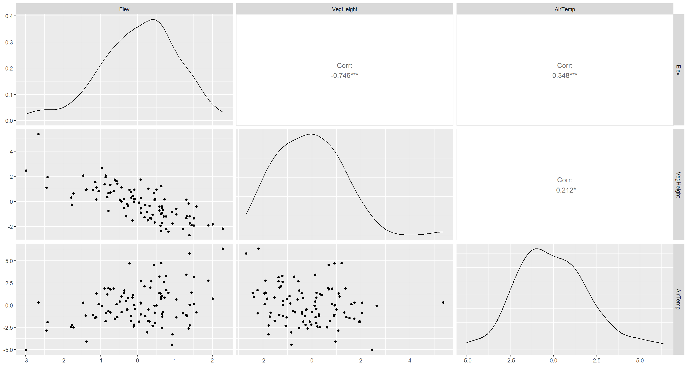
First, I need to show that there even is a (spurious) association between vegetation height (VegHeight) and air temperature (AirTemp):
m <- quap(
  alist(
    VegHeight ~ dnorm(mu, sigma),
    mu <- a + bAT * AirTemp,
    a ~ dnorm(0, 1),
    bAT ~ dnorm(0, 1),
    sigma ~ dunif(0, 2)
  ),
  data = d
)
precis(m)
##             mean         sd       5.5%       94.5%
## a     -0.1163981 0.13088036 -0.3255702  0.09277397
## bAT   -0.1334516 0.06168793 -0.2320409 -0.03486242
## sigma  1.3201363 0.09334783  1.1709484  1.46932412
Next, let’s see what happens when I add elevation data (Elev):
m <- quap(
  alist(
    VegHeight ~ dnorm(mu, sigma),
    mu <- a + bAT * AirTemp + bEL * Elev,
    a ~ dnorm(0, 1),
    bAT ~ dnorm(0, 1),
    bEL ~ dnorm(0, 1),
    sigma ~ dunif(0, 2)
  ),
  data = d
)
precis(m)
##              mean         sd        5.5%      94.5%
## a     -0.08752358 0.08934620 -0.23031606  0.0552689
## bAT    0.03291017 0.04470657 -0.03853957  0.1043599
## bEL   -0.98905981 0.09190458 -1.13594107 -0.8421785
## sigma  0.89659689 0.06340391  0.79526519  0.9979286
Conclusively, according to our simulated data and the multiple regression analysis, increasing elevation leads to decreased vegetation height directly. Since the bivariate effect of decreasing air temperature leading to decreases in vegetation height vanishes when we include elevation data, we deem this association to be spurious.
Practice M2
Question: Invent your own example of a masked relationship. An outcome variable should be correlated with both predictor variables, but in opposite directions. And the two predictor variables should be correlated with one another.
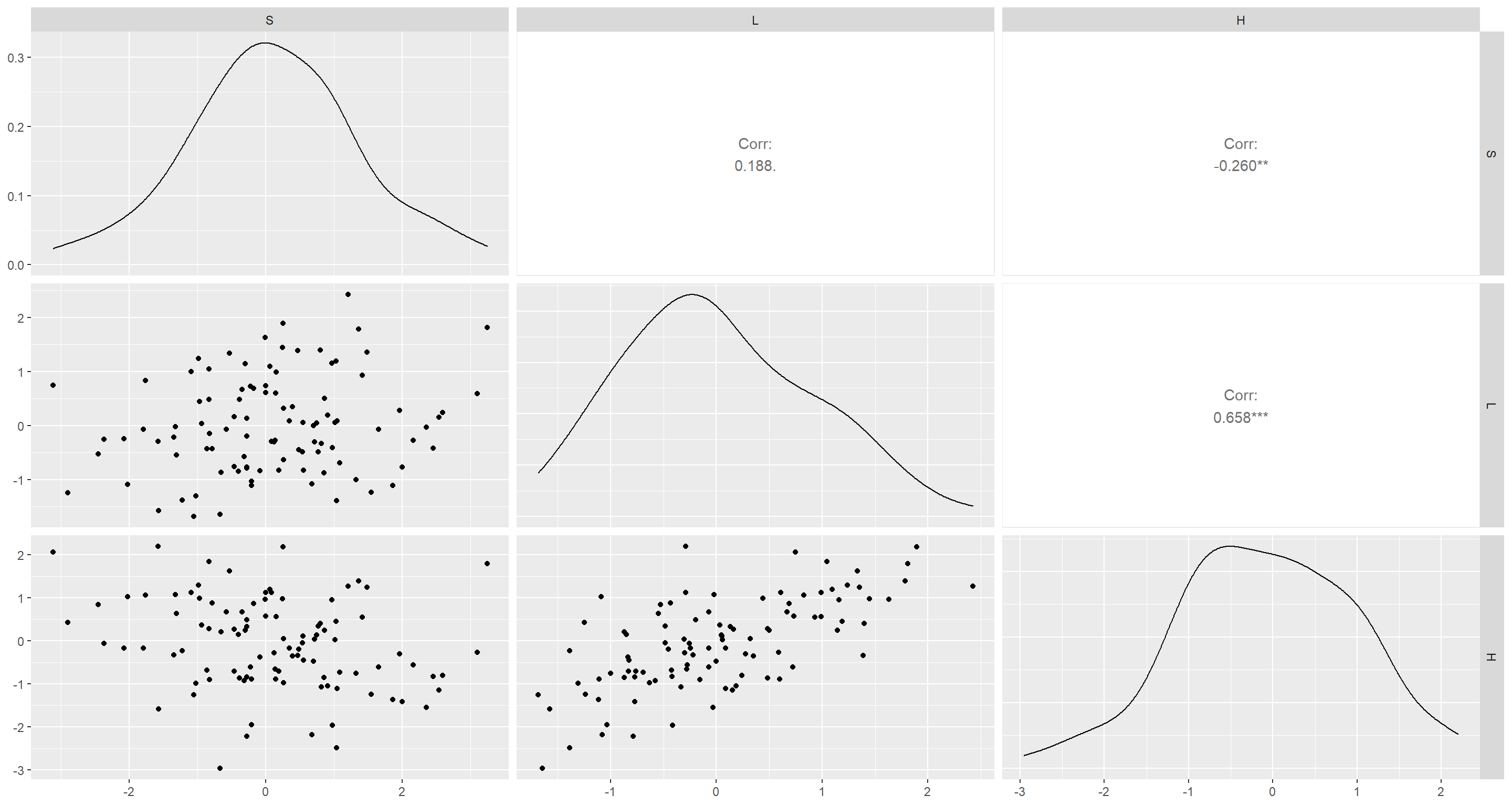
Answer: Again, I take inspiration from an Overthinking box. This time from page 156. Here, I create an example of of species richness (S) as driven by human footprint (H), and latitude centred on the equator (L).
N <- 1e2
rho <- 0.6
L <- rnorm(n = N, mean = 0, sd = 1)
H <- rnorm(n = N, mean = rho * L, sd = sqrt(1 - rho^2))
S <- rnorm(n = N, mean = L - H, sd = 1)
d <- data.frame(S, L, H)
ggpairs(d)
Let’s start with some bivariate models:
## Latitude centred on equator
m1 <- quap(
  alist(
    S ~ dnorm(mu, sigma),
    mu <- a + bL * L,
    a ~ dnorm(0, 1),
    bL ~ dnorm(0, 1),
    sigma ~ dunif(0, 2)
  ),
  data = d
)
precis(m1)
##             mean         sd        5.5%     94.5%
## a     0.09656591 0.12275009 -0.09961245 0.2927443
## bL    0.26165086 0.13796469  0.04115663 0.4821451
## sigma 1.23678173 0.08745475  1.09701214 1.3765513
## Human footprint
m2 <- quap(
  alist(
    S ~ dnorm(mu, sigma),
    mu <- a + bH * H,
    a ~ dnorm(0, 1),
    bH ~ dnorm(0, 1),
    sigma ~ dunif(0, 2)
  ),
  data = d
)
precis(m2)
##              mean        sd       5.5%      94.5%
## a      0.07758373 0.1209797 -0.1157652  0.2709327
## bH    -0.30689555 0.1147838 -0.4903422 -0.1234489
## sigma  1.21600759 0.0859864  1.0785847  1.3534305
Finally, let’s combine these into one big multiple regression:
m3 <- quap(
  alist(
    S ~ dnorm(mu, sigma),
    mu <- a + bH * H + bL * L,
    a ~ dnorm(0, 1),
    bH ~ dnorm(0, 1),
    bL ~ dnorm(0, 1),
    sigma ~ dunif(0, 2)
  ),
  data = d
)
precis(m3)
##              mean         sd       5.5%      94.5%
## a      0.03603387 0.10567367 -0.1328531  0.2049208
## bH    -0.78399406 0.13167742 -0.9944400 -0.5735481
## bL     0.86622135 0.15576555  0.6172779  1.1151648
## sigma  1.05757879 0.07482312  0.9379970  1.1771606
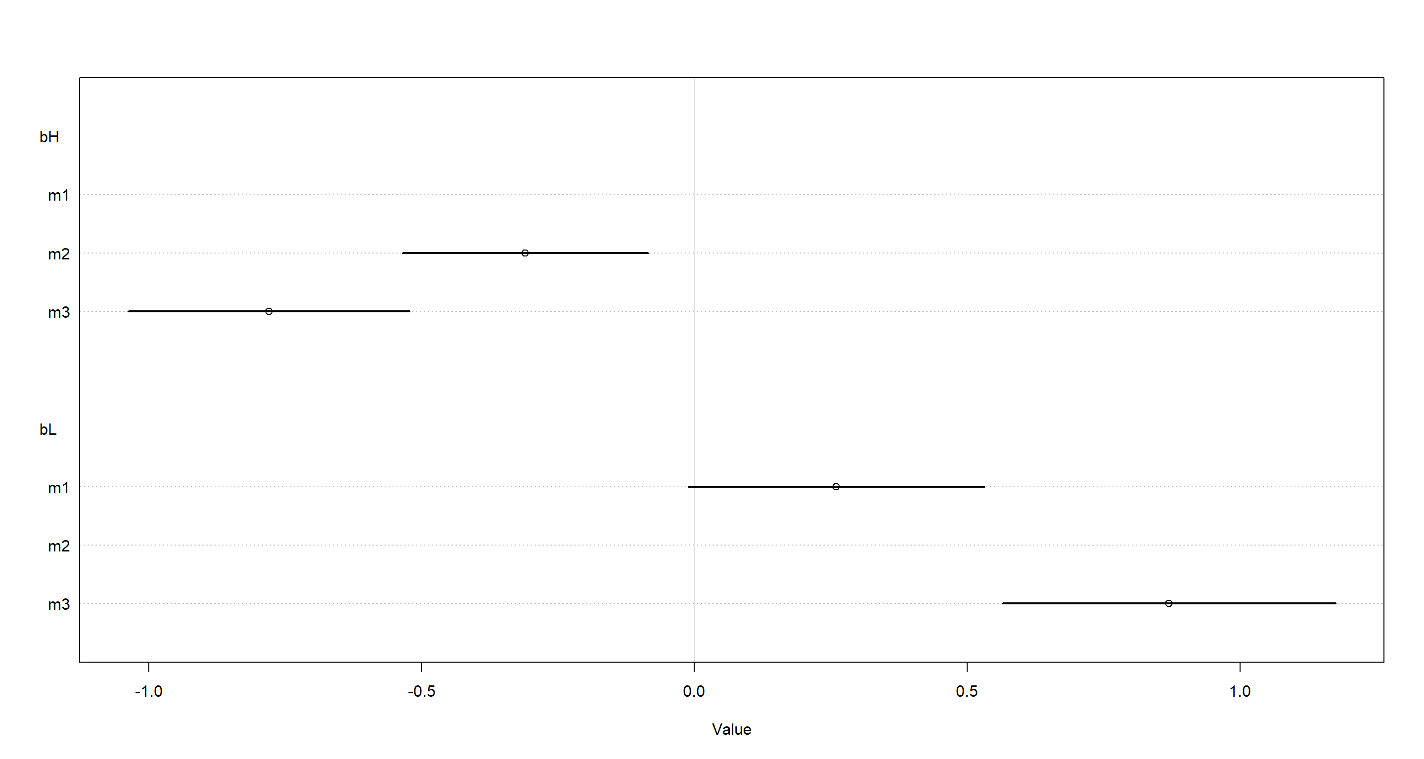
Both associations became stronger! To link this back to reality, equatoward position has been linked to increased species richness for a long time (through many hypotheses I won’t go into here), there is also a global pattern of reduced human footprint around the equator (although this may change… looking at you, Brazil). Human footprint itself has been unequivocally linked with a decrease in species richness.
Let’s look at this in plotted form:
plot(coeftab(m3, m2, m1), par = c("bH", "bL"))
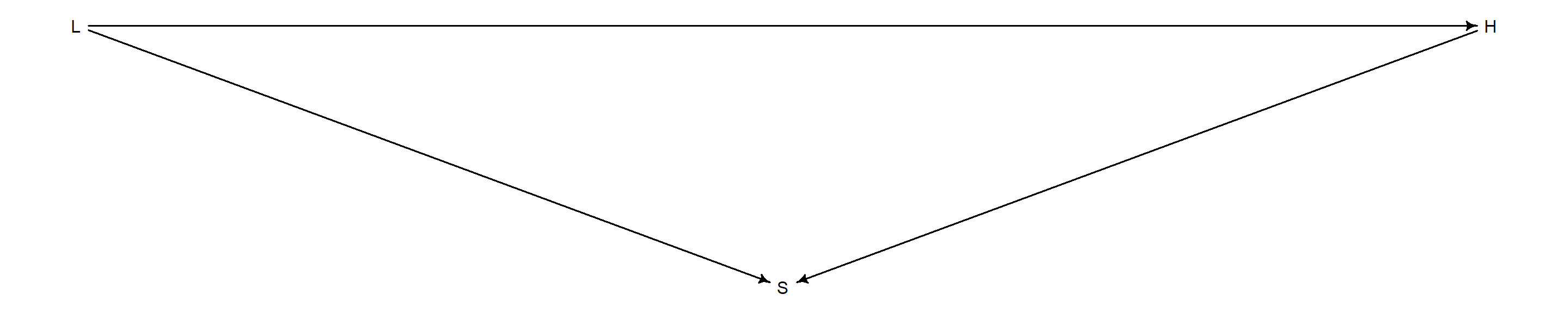
In a Directed Acyclic Graph, this works out to:
dag <- dagitty("dag { L -> S L -> H H -> S}")
coordinates(dag) <- list(x = c(L = 0, S = 1, H = 2), y = c(L = 0, S = 1, H = 0))
drawdag(dag)
Practice M3
Question: It is sometimes observed that the best predictor of fire risk is the presence of firefighters - States and localities with many firefighters also have more fires. Presumably firefighters do not cause fires. Nevertheless, this is not a spurious correlation. Instead fires cause firefighters. Consider the same reversal of causal inference in the context of the divorce and marriage data. How might a high divorce rate cause a higher marriage rate? Can you think of a way to evaluate this relationship, using multiple regression?
Answer: Divorces introduce un-married individuals to the population. These individuals have already demonstrated a readiness to get married in the first place and so might spike marriage rates via re-marrying. I would test for this by running a multiple regression in which I regress marriage rate on divorce rate and re-marriage rate (this excludes first-marriages). As long as divorce no longer predicts marriage rate once re-marriage rate is known, our hypothesis would be true.
Practice M4
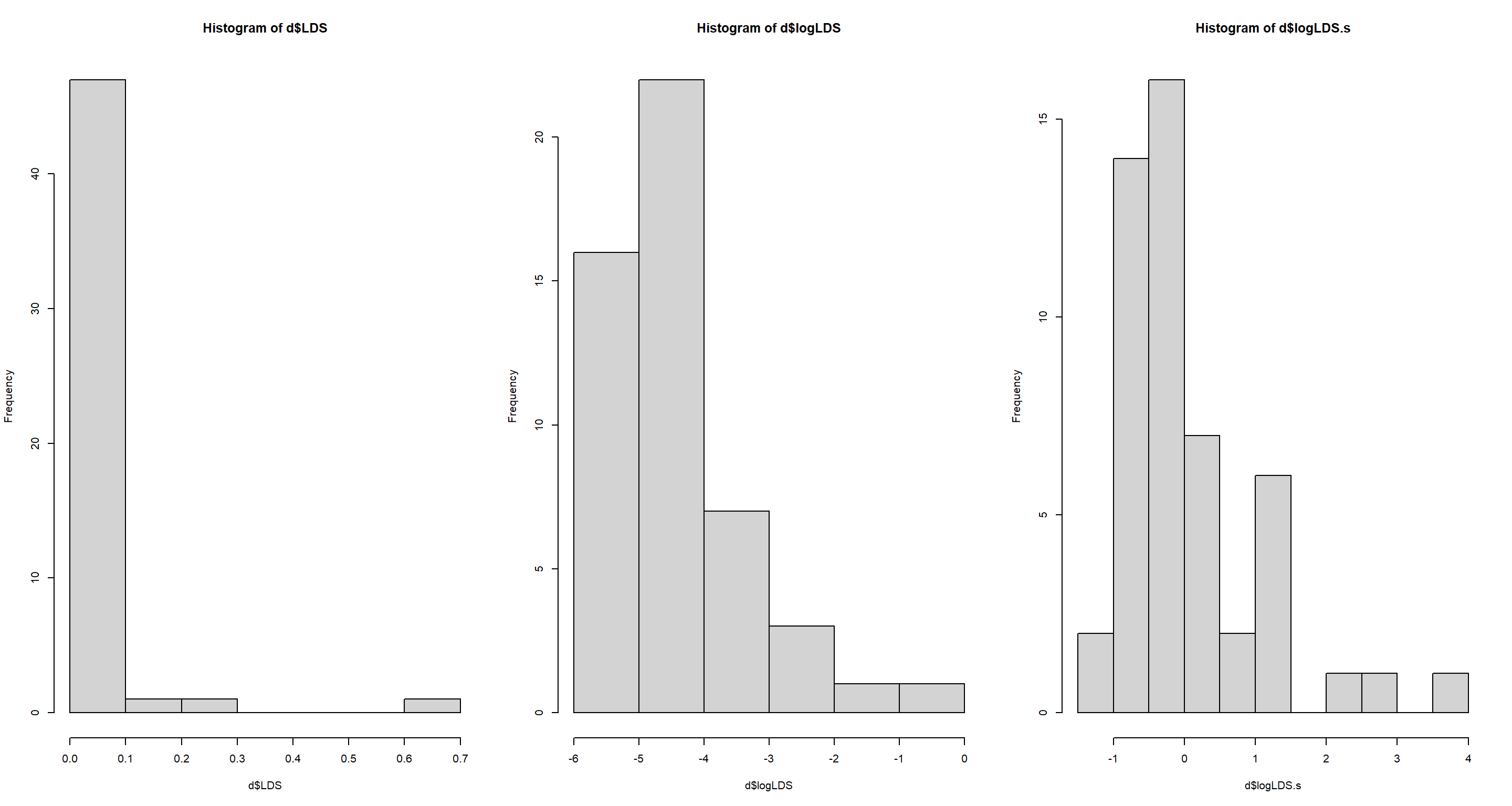
Question: In the divorce data, States with high numbers of Mormons (members of The Church of Jesus Christ of Latter-day Saints, LDS) have much lower divorce rates than the regression models expected. Find a list of LDS population by State and use those numbers as a predictor variable, predicting divorce rate using marriage rate, median age at marriage, and percent LDS population (possibly standardised). You may want to consider transformations of the raw percent LDS variable.
Answer: Here, I use the percentage values of LDS as obtained through Wikipedia by Jeffrey Girard. Since there is a large skew in these data due to states with large LDS populations, I apply a log-transformation before standardising:
data("WaffleDivorce")
d <- WaffleDivorce
d$LDS <- c(0.0077, 0.0453, 0.0610, 0.0104, 0.0194, 0.0270, 0.0044, 0.0057, 0.0041, 0.0075, 0.0082, 0.0520, 0.2623, 0.0045, 0.0067, 0.0090, 0.0130, 0.0079, 0.0064, 0.0082, 0.0072, 0.0040, 0.0045, 0.0059, 0.0073, 0.0116, 0.0480, 0.0130, 0.0065, 0.0037, 0.0333, 0.0041, 0.0084, 0.0149, 0.0053, 0.0122, 0.0372, 0.0040, 0.0039, 0.0081, 0.0122, 0.0076, 0.0125, 0.6739, 0.0074, 0.0113, 0.0390, 0.0093, 0.0046, 0.1161)
d$logLDS <- log(d$LDS)
d$logLDS.s <- (d$logLDS - mean(d$logLDS)) / sd(d$logLDS)
par(mfrow = c(1, 3))
hist(d$LDS)
hist(d$logLDS)
hist(d$logLDS.s)
Now I am ready to build the model:
m <- map(
  alist(
    Divorce ~ dnorm(mu, sigma),
    mu <- a + bm * Marriage + ba * MedianAgeMarriage + bl * logLDS.s,
    a ~ dnorm(10, 20),
    bm ~ dnorm(0, 10),
    ba ~ dnorm(0, 10),
    bl ~ dnorm(0, 10),
    sigma ~ dunif(0, 5)
  ),
  data = d
)
precis(m)
##              mean         sd      5.5%      94.5%
## a     35.43051636 6.77505687 24.602667 46.2583658
## bm     0.05343619 0.08261404 -0.078597  0.1854694
## ba    -1.02939820 0.22468646 -1.388491 -0.6703058
## bl    -0.60777261 0.29055419 -1.072134 -0.1434109
## sigma  1.37864526 0.13836923  1.157505  1.5997860
While marriage rate is not a powerful predictor of divorce rate, both age at marriage and percentage of LDS population are strongly negatively associated with divorce rates.
Practice M5
Question: One way to reason through multiple causation hypotheses is to imagine detailed mechanisms through which predictor variables may influence outcomes. For example, it is sometimes argued that the price of gasoline (predictor variable) is positively associated with lower obesity rates (outcome variable). However, there are at least two important mechanisms by which the price of gas could reduce obesity. First, it could lead to less driving and therefore more exercise. Second, it could lead to less driving, which leads to less eating out, which leads to less consumption of huge restaurant meals. Can you outline one or more multiple regressions that address these two mechanisms? Assume you can have any predictor data you need.
Answer: $μ_i=α+β_GG_i+β_EE_i+β_RR_i$. I propose we run a multiple regression containing a variable $E$ denoting frequency of exercising, and another variable $R$ which captures the frequency of restaurant visits. We use these alongside the variable $G$ (gasoline price) to model obesity rates.
Hard Exercises
Disclaimer: All three exercises below use the same data, data(foxes) (part of rethinking). The urban fox (Vulpes vulpes) is a successful exploiter of human habitat. Since urban foxes move in packs and defend territories, data on habitat quality and population density is also included. The data frame has five columns:
(1) group: Number of the social group the individual fox belongs to
(2) avgfood: The average amount of food available in the territory
(3) groupsize: The number of foxes in the social group
(4) area: Size of the territory
(5) weight: Body weight of the individual fox
data("foxes")
Practice H1
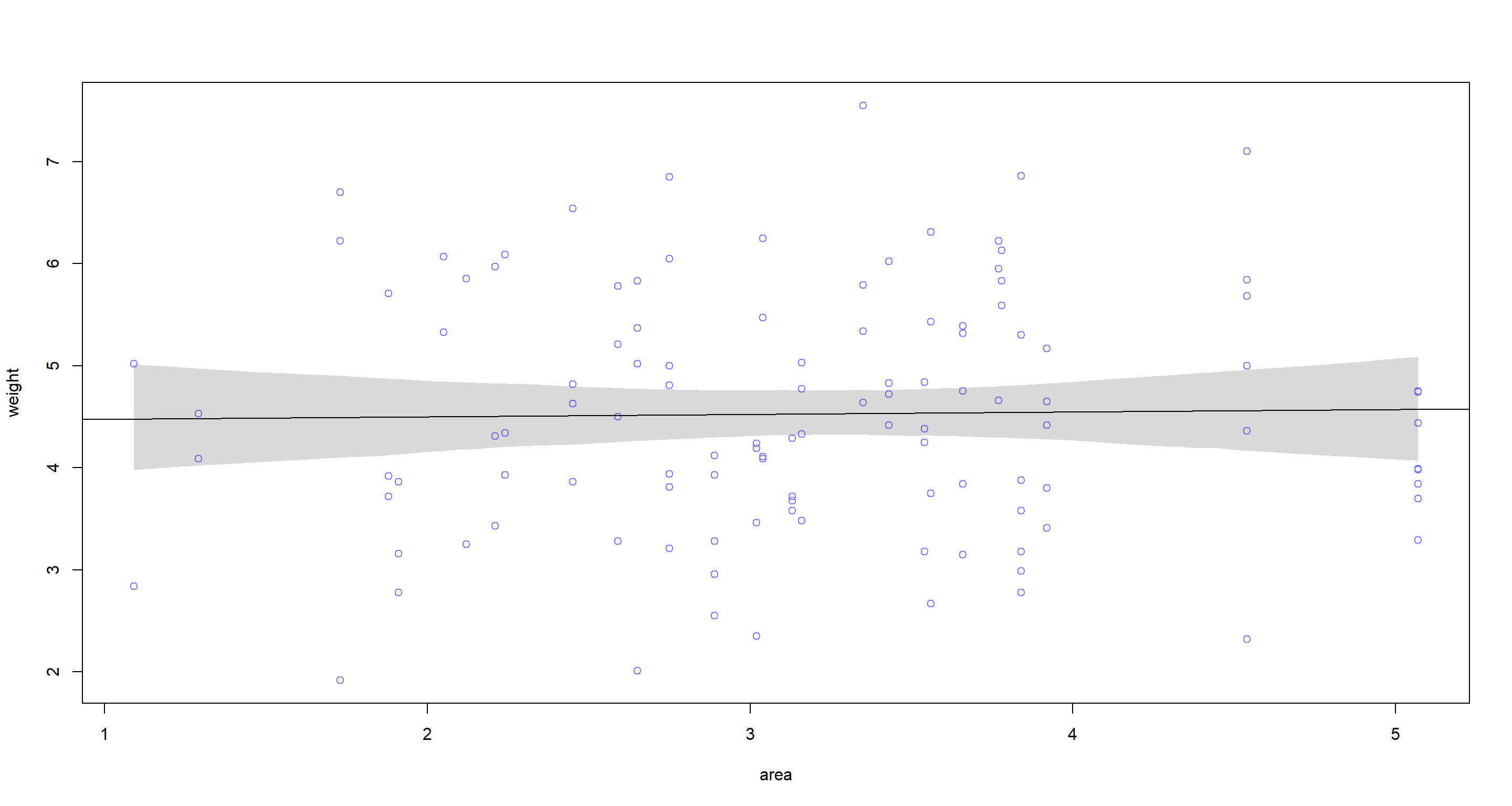
Question: Fit two bivariate Gaussian regressions, using quap: (1) body weight as a linear function of territory size (area), and (2) body weight as a linear function of groupsize. Plot the results of these regressions, displaying the MAP regression line and the 95% interval of the mean. Is either variable important for predicting fox body weight?
Answer: Let’s start with the models:
## Area
d <- foxes
ma <- quap(
  alist(
    weight ~ dnorm(mu, sigma),
    mu <- a + ba * area,
    a ~ dnorm(5, 5),
    ba ~ dnorm(0, 5),
    sigma ~ dunif(0, 5)
  ),
  data = d
)
precis(ma)
##             mean         sd       5.5%     94.5%
## a     4.45430638 0.38955723  3.8317187 5.0768941
## ba    0.02385824 0.11803080 -0.1647778 0.2124943
## sigma 1.17868417 0.07738415  1.0550093 1.3023590
area.seq <- seq(from = min(d$area), to = max(d$area), length.out = 1e4)
mu <- link(ma, data = data.frame(area = area.seq))
mu.PI <- apply(mu, 2, PI, prob = 0.95)
plot(weight ~ area, data = d, col = rangi2)
abline(ma)
shade(mu.PI, area.seq)
## Group Size
mg <- quap(
  alist(
    weight ~ dnorm(mu, sigma),
    mu <- a + bg * groupsize,
    a ~ dnorm(5, 5),
    bg ~ dnorm(0, 5),
    sigma ~ dunif(0, 5)
  ),
  data = d
)
precis(mg)
##             mean         sd       5.5%       94.5%
## a      5.0675829 0.32418282  4.5494762  5.58568969
## bg    -0.1238161 0.07038361 -0.2363027 -0.01132946
## sigma  1.1635303 0.07638932  1.0414454  1.28561522
groupsize.seq <- seq(from = min(d$groupsize), to = max(d$groupsize), length.out = 1e4)
mu <- link(mg, data = data.frame(groupsize = groupsize.seq))
mu.PI <- apply(mu, 2, PI, prob = 0.95)
plot(weight ~ groupsize, data = d, col = rangi2)
abline(mg)
shade(mu.PI, groupsize.seq)
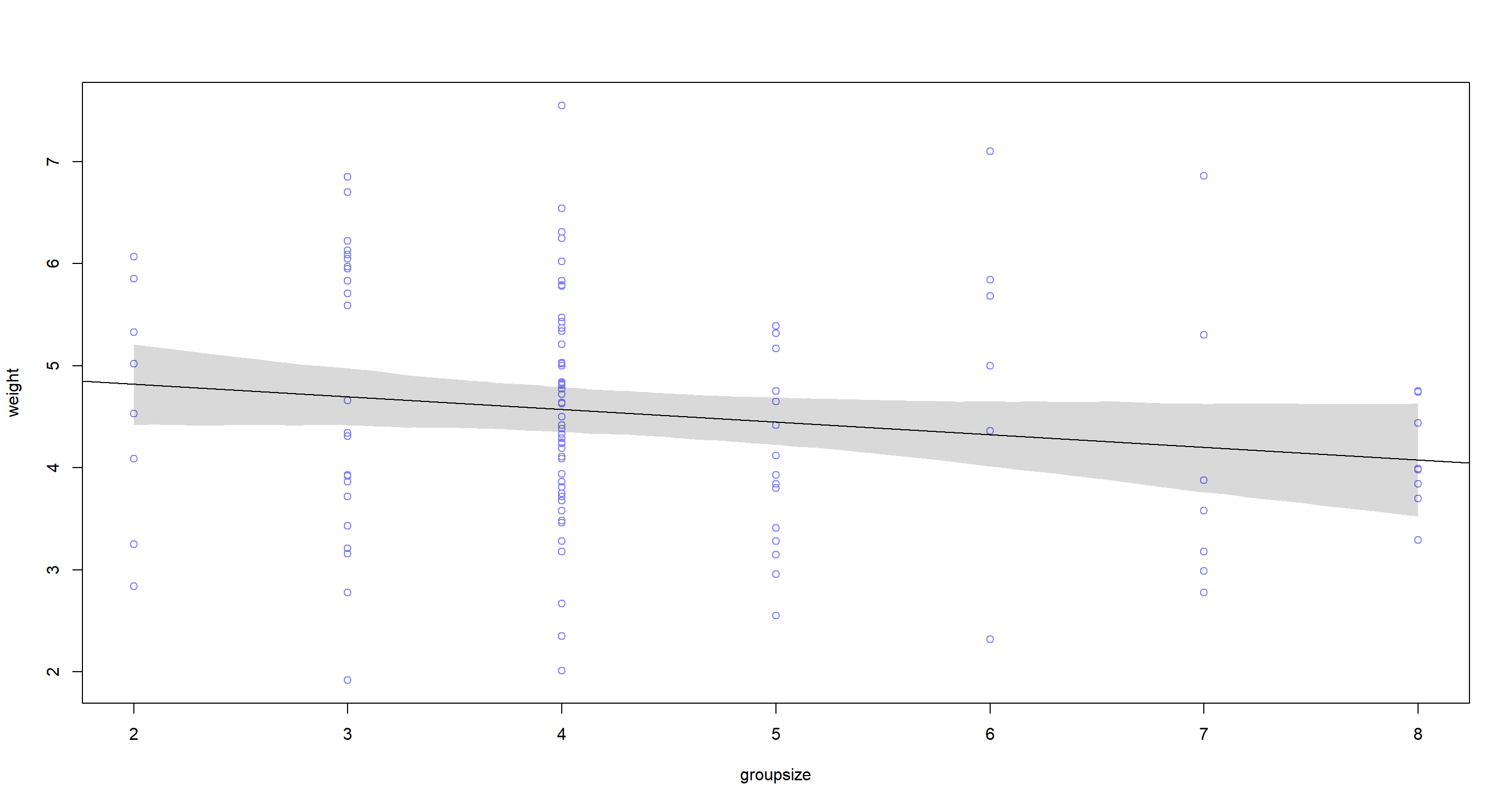
According to these two bivariate models, neither area nor groupsize have strong associations with weight of which we could be certain.
Practice H2
Question: Now fit a multiple linear regression with weight as the outcome and both area and groupsize as predictor variables. Plot the predictions of the model for each predictor, holding the other predictor constant at its mean. What does this model say about the importance of each variable? Why do you get different results than you got in the exercise just above?
Answer: First, we run the model itself:
mag <- quap(
  alist(
    weight ~ dnorm(mu, sigma),
    mu <- a + ba * area + bg * groupsize,
    a ~ dnorm(5, 5),
    ba ~ dnorm(0, 5),
    bg ~ dnorm(0, 5),
    sigma ~ dunif(0, 5)
  ),
  data = d
)
precis(mag)
##             mean         sd       5.5%      94.5%
## a      4.4541696 0.36977162  3.8632031  5.0451360
## ba     0.6159473 0.19978363  0.2966545  0.9352402
## bg    -0.4318471 0.12066677 -0.6246959 -0.2389982
## sigma  1.1184516 0.07342985  1.0010965  1.2358067
Now, I want to actually have a look at the underlying data:
ggpairs(d[, 3:5])
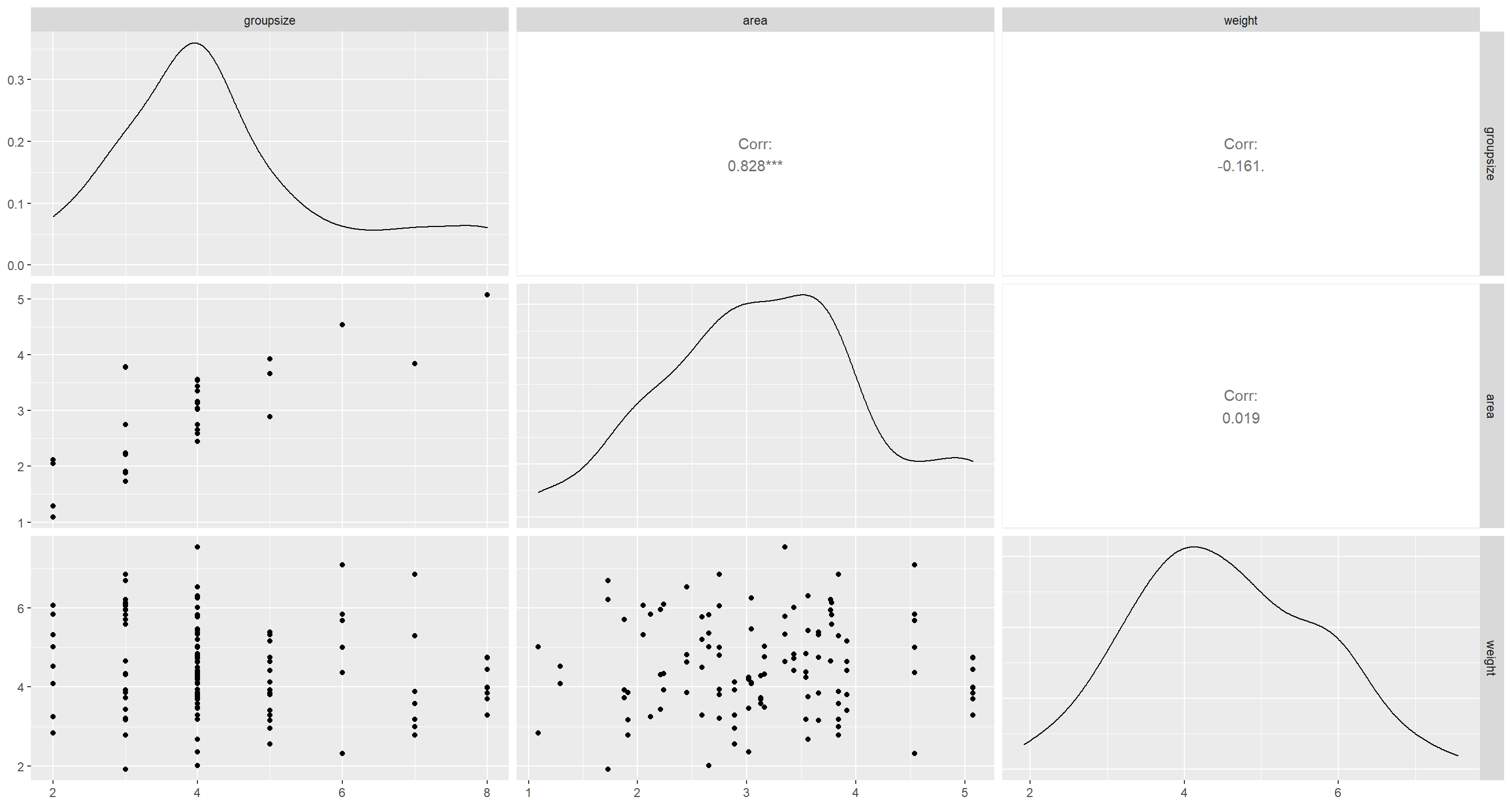
groupsize and area are pretty heavily associated it seems. Finally, we establish counterfactual plots:
## Fixing Group Size
G.avg <- mean(d$groupsize)
A.seq <- seq(from = 0, to = 6, length.out = 1e4)
pred.data <- data.frame(
groupsize = G.avg,
area = A.seq
)
mu <- link(mag, data = pred.data)
mu.mean <- apply(mu, 2, mean)
mu.PI <- apply(mu, 2, PI, prob = 0.95)
A.sim <- sim(mag, data = pred.data, n = 1e4)
A.PI <- apply(A.sim, 2, PI)
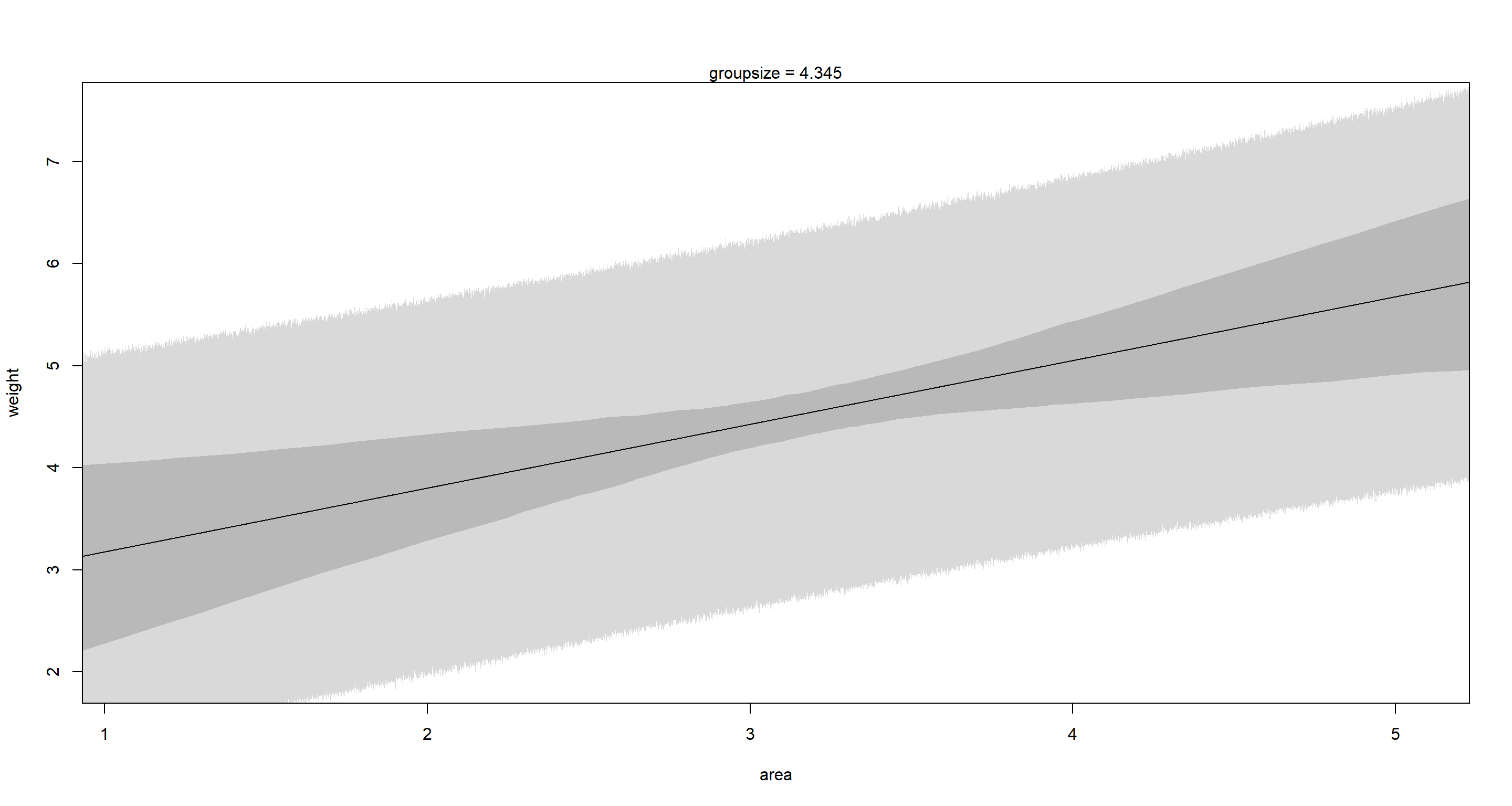
plot(weight ~ area, data = d, type = "n")
mtext("groupsize = 4.345")
lines(A.seq, mu.mean)
shade(mu.PI, A.seq)
shade(A.PI, A.seq)
## Fixing Area
A.avg <- mean(d$area)
G.seq <- seq(from = 1, to = 10, length.out = 1e4)
pred.data <- data.frame(
  groupsize = G.seq,
  area = A.avg
)
mu <- link(mag, data = pred.data)
mu.mean <- apply(mu, 2, mean)
mu.PI <- apply(mu, 2, PI, prob = 0.95)
G.sim <- sim(mag, data = pred.data, n = 1e4)
G.PI <- apply(G.sim, 2, PI)
plot(weight ~ groupsize, data = d, type = "n")
mtext("area = 3.169")
lines(G.seq, mu.mean)
shade(mu.PI, G.seq)
shade(G.PI, G.seq)
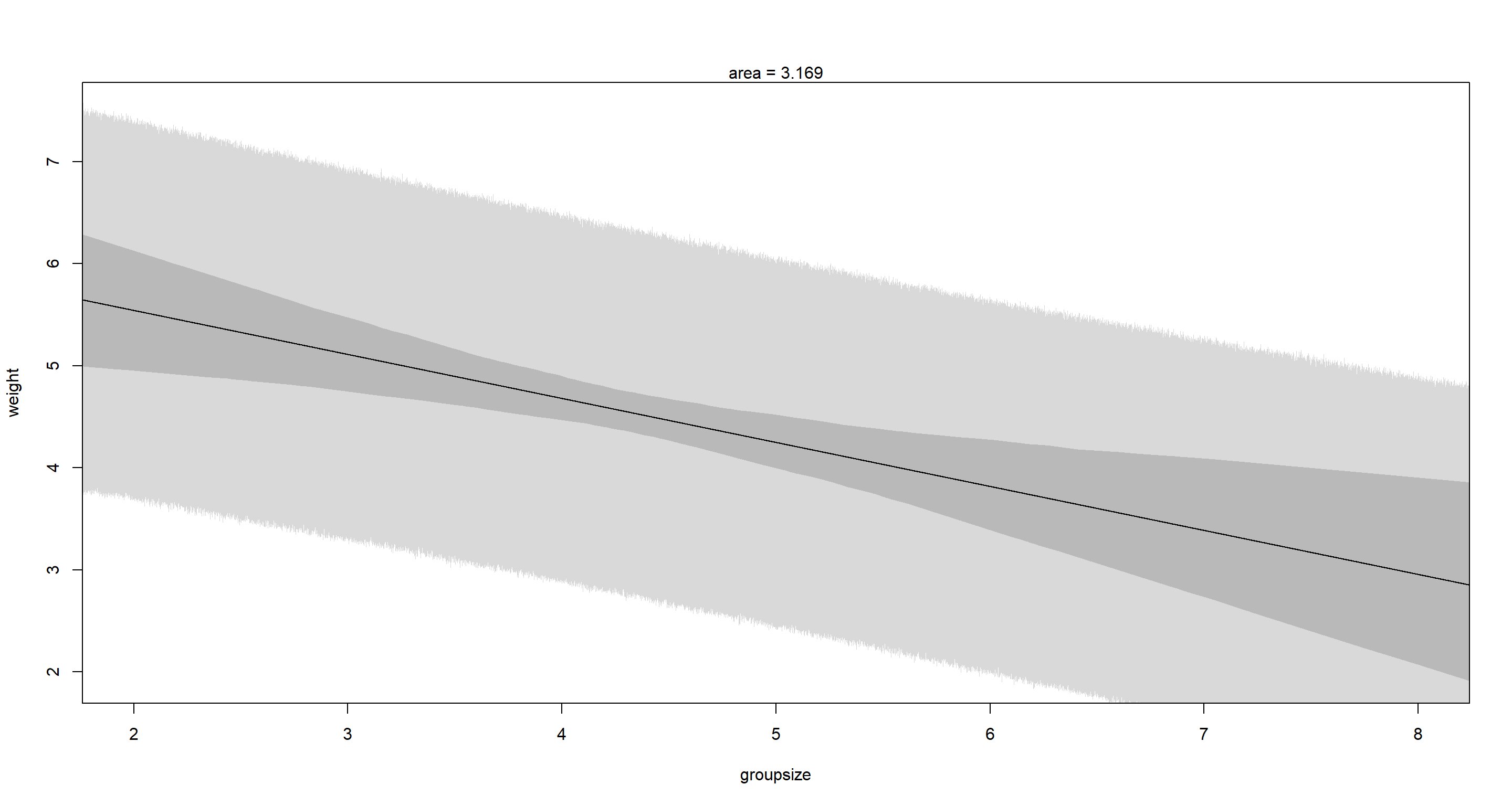
This is a clear example of a masking relationship. When considered in isolation (bivariate models) neither groupsize nor area show clear associations with weight. However, as soon as we use a multiple regression, we find that weight declines as groupsize increases, while area has the opposite effect. These effects cancel each other out in bivariate settings.
Practice H3
Question: Finally, consider the avgfood variable. Fit two more multiple regressions: (1) body weight as an additive function of avgfood and groupsize, and (2) body weight as an additive function of all three variables, avgfood and groupsize and area. Compare the results of these models to the previous models you’ve fit, in the first two exercises.
Answer: First, we require the model with two variables:
m <- quap(
  alist(
    weight ~ dnorm(mu, sigma),
    mu <- a + bf * avgfood + bg * groupsize,
    a ~ dnorm(5, 5),
    bf ~ dnorm(0, 5),
    bg ~ dnorm(0, 5),
    sigma ~ dunif(0, 5)
  ),
  data = d
)
precis(m)
##             mean         sd       5.5%      94.5%
## a      4.1806405 0.42501186  3.5013895  4.8598915
## bf     3.6052545 1.17683527  1.7244445  5.4860646
## bg    -0.5433458 0.15271144 -0.7874082 -0.2992834
## sigma  1.1166611 0.07332213  0.9994782  1.2338441
Next, we need the model with three variables:
m <- quap(
  alist(
    weight ~ dnorm(mu, sigma),
    mu <- a + bf * avgfood + bg * groupsize + ba * area,
    a ~ dnorm(5, 5),
    bf ~ dnorm(0, 5),
    bg ~ dnorm(0, 5),
    ba ~ dnorm(0, 5),
    sigma ~ dunif(0, 5)
  ),
  data = d
)
precis(m)
##             mean         sd        5.5%      94.5%
## a      4.1010815 0.42308541  3.42490933  4.7772537
## bf     2.3024285 1.39359133  0.07520038  4.5296566
## bg    -0.5926614 0.15385399 -0.83854977 -0.3467730
## ba     0.4017410 0.23609446  0.02441642  0.7790655
## sigma  1.1044452 0.07252194  0.98854116  1.2203493
Part A
Question: Is avgfood or area a better predictor of body weight? If you had to choose one or the other to include in a model, which would it be? Support your assessment with any tables or plots you choose.
Answer: According to intuition, I would prefer avgfood because it is directly and obviously linked to a gain in calories and thus weight whereas area is a fairly indirect relationship. However, I still want to test this in R. Let’s first look at the raw data:
ggpairs(d[, -1])
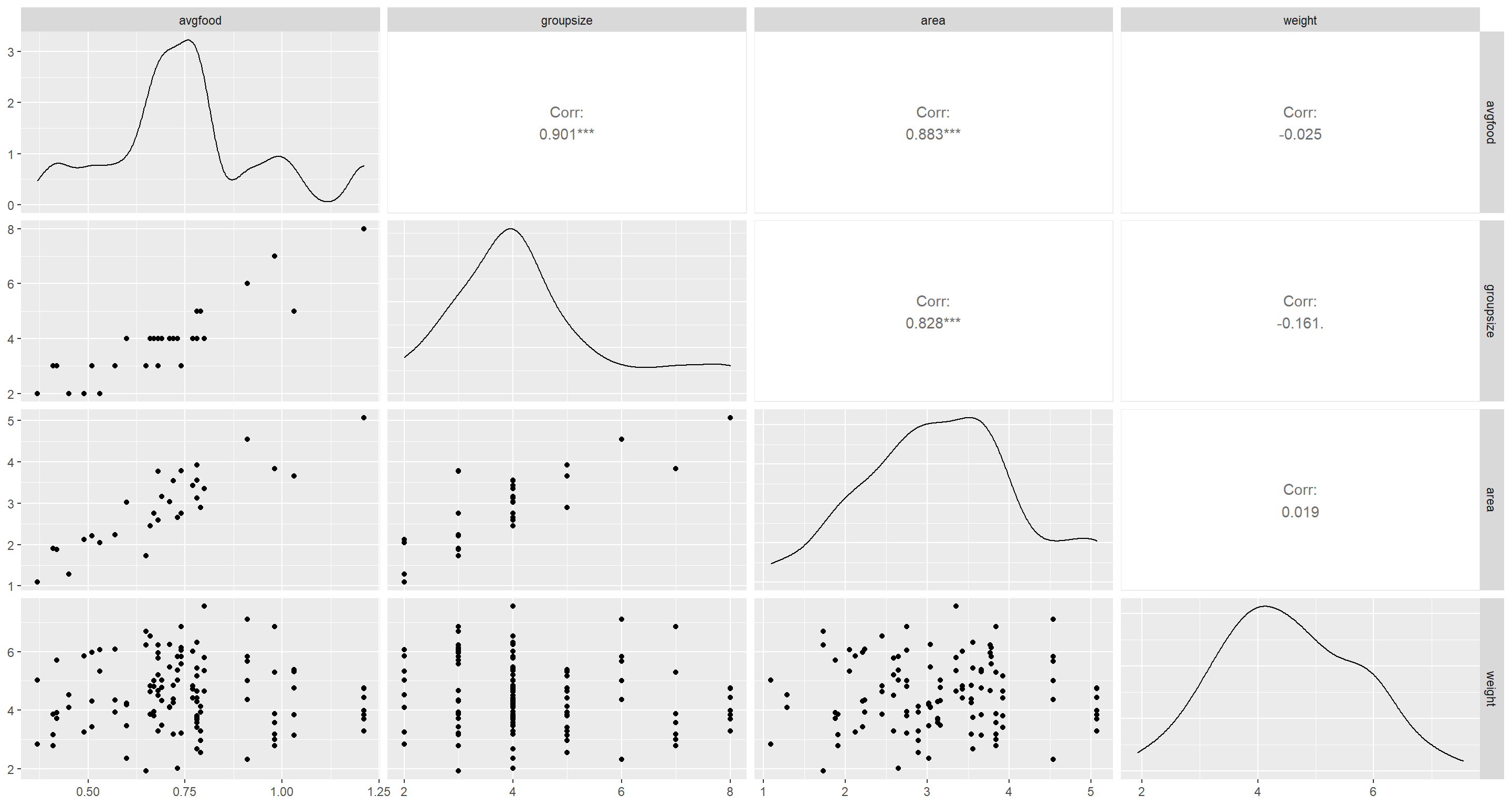
avgfood and area are strikingly correlated with one another. To chose the most informative of these two, I build models of weight solely dependant on standardised records of both (so the slope estimates are comparable in their magnitude) as well as groupsize:
## Average Food
d$avgfood.s <- (d$avgfood - mean(d$avgfood)) / sd(d$avgfood)
m <- quap(
  alist(
    weight ~ dnorm(mu, sigma),
    mu <- a + bf * avgfood.s + bg * groupsize,
    a ~ dnorm(5, 5),
    bf ~ dnorm(0, 5),
    bg ~ dnorm(0, 5),
    sigma ~ dunif(0, 5)
  ),
  data = d
)
precis(m)
##             mean         sd       5.5%      94.5%
## a      6.9566906 0.67995576  5.8699900  8.0433913
## bf     0.7450529 0.23844151  0.3639773  1.1261284
## bg    -0.5588002 0.15473498 -0.8060966 -0.3115038
## sigma  1.1166194 0.07331182  0.9994530  1.2337859
## Area
d$area.s <- (d$area - mean(d$area)) / sd(d$area)
m <- quap(
  alist(
    weight ~ dnorm(mu, sigma),
    mu <- a + ba * area.s + bg * groupsize,
    a ~ dnorm(5, 5),
    ba ~ dnorm(0, 5),
    bg ~ dnorm(0, 5),
    sigma ~ dunif(0, 5)
  ),
  data = d
)
precis(m)
##             mean         sd       5.5%      94.5%
## a      6.3903420 0.53148096  5.5409327  7.2397512
## ba     0.5682683 0.18494820  0.2726854  0.8638512
## bg    -0.4283914 0.12001993 -0.6202064 -0.2365764
## sigma  1.1184575 0.07343099  1.0011006  1.2358144
Given these results, I prefer the stronger relationship between weight and avgfood over that relying on area and would chose a model using only avgfood.
Part B
Question: When both avgfood or area are in the same model, their effects are reduced (closer to zero) and their standard errors are larger than when they are included in separate models. Can you explain this result?
Answer: I am pretty sure that this is our old friend multicollinearity rearing its ugly head. Since the two are highly correlated, their respective effects become less when controlling for either in the same model.
Session Info
sessionInfo()
## R version 4.0.5 (2021-03-31)
## Platform: x86_64-w64-mingw32/x64 (64-bit)
## Running under: Windows 10 x64 (build 19043)
##
## Matrix products: default
##
## locale:
## [1] LC_COLLATE=English_United Kingdom.1252  LC_CTYPE=English_United Kingdom.1252    LC_MONETARY=English_United Kingdom.1252 LC_NUMERIC=C
## [5] LC_TIME=English_United Kingdom.1252
##
## attached base packages:
## [1] parallel  stats     graphics  grDevices utils     datasets  methods   base
##
## other attached packages:
## [1] dagitty_0.3-1        GGally_2.1.2         rethinking_2.13      rstan_2.21.2         ggplot2_3.3.6        StanHeaders_2.21.0-7
##
## loaded via a namespace (and not attached):
##  [1] Rcpp_1.0.7         mvtnorm_1.1-1      lattice_0.20-41    prettyunits_1.1.1  ps_1.6.0           assertthat_0.2.1   digest_0.6.27      utf8_1.2.1         V8_3.4.1           plyr_1.8.6
## [11] R6_2.5.0           backports_1.2.1    stats4_4.0.5       evaluate_0.14      coda_0.19-4        highr_0.9          blogdown_1.3       pillar_1.6.0       rlang_0.4.11       curl_4.3.2
## [21] callr_3.7.0        jquerylib_0.1.4    R.utils_2.10.1     R.oo_1.24.0        rmarkdown_2.7      styler_1.4.1       labeling_0.4.2     stringr_1.4.0      loo_2.4.1          munsell_0.5.0
## [31] compiler_4.0.5     xfun_0.22          pkgconfig_2.0.3    pkgbuild_1.2.0     shape_1.4.5        htmltools_0.5.1.1  tidyselect_1.1.0   tibble_3.1.1       gridExtra_2.3      bookdown_0.22
## [41] codetools_0.2-18   matrixStats_0.61.0 reshape_0.8.8      fansi_0.4.2        crayon_1.4.1       dplyr_1.0.5        withr_2.4.2        MASS_7.3-53.1      R.methodsS3_1.8.1  grid_4.0.5
## [51] jsonlite_1.7.2     gtable_0.3.0       lifecycle_1.0.0    DBI_1.1.1          magrittr_2.0.1     scales_1.1.1       RcppParallel_5.1.2 cli_3.0.0          stringi_1.5.3      farver_2.1.0
## [61] bslib_0.2.4        ellipsis_0.3.2     generics_0.1.0     vctrs_0.3.7        boot_1.3-27        rematch2_2.1.2     RColorBrewer_1.1-2 tools_4.0.5        R.cache_0.14.0     glue_1.4.2
## [71] purrr_0.3.4        processx_3.5.1     yaml_2.2.1         inline_0.3.17      colorspace_2.0-0   knitr_1.33         sass_0.3.1