A Primer For Statistical Tests

Theory

These are the solutions to the exercises contained within the handout to A Primer For Statistical Tests which walks you through the basics of variables, their scales and distributions. Keep in mind that there is probably a myriad of other ways to reach the same conclusions as presented in these solutions.

Data

Find the data for this exercise here.

Loading the R Environment Object

load("Data/Primer.RData")  # load data file from Data folder

Variables

Finding Variables

ls()  # list all elements in working environment

## [1] "Colour"               "Depth"                "IndividualsPassingBy"
## [4] "Length"               "Reproducing"          "Sex"                 
## [7] "Size"                 "Temperature"

Colour

class(Colour)  # mode

## [1] "character"

barplot(table(Colour))  # fitting?

Question	Answer
Mode?	character
Which scale?	Nominal
What’s implied?	Categorical data that can’t be ordered
Does data fit scale?	Yes

Depth

class(Depth)  # mode

## [1] "numeric"

barplot(Depth)  # fitting?

Question	Answer
Mode?	numeric
Which scale?	Interval/Discrete
What’s implied?	Continuous data with a non-absence point of origin
Does data fit scale?	Debatable (is 0 depth absence of depth?)

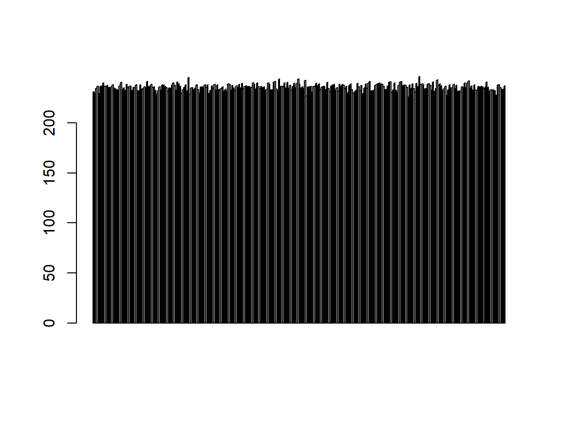
IndividualsPassingBy

class(IndividualsPassingBy)  # mode

## [1] "integer"

barplot(IndividualsPassingBy)  # fitting?

Question	Answer
Mode?	integer
Which scale?	Integer
What’s implied?	Only integer numbers with an absence point of origin
Does data fit scale?	Yes

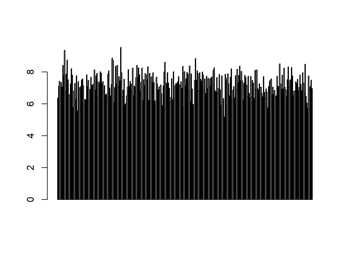
Length

class(Length)  # mode

## [1] "numeric"

barplot(Length)  # fitting?

Question	Answer
Mode?	numeric
Which scale?	Relation/Ratio
What’s implied?	Continuous data with an absence point of origin
Does data fit scale?	Yes

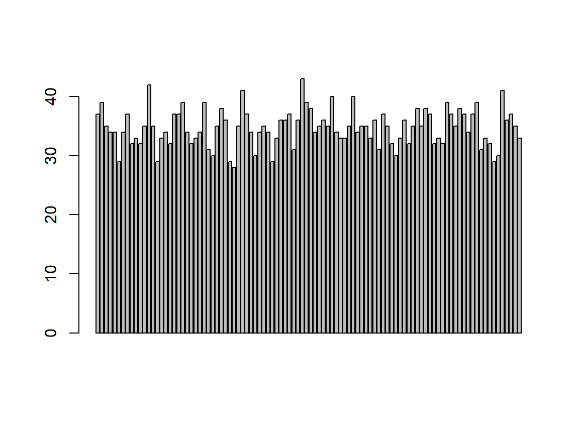
Reproducing

class(Reproducing)  # mode

## [1] "integer"

barplot(Reproducing)  # fitting?

Question	Answer
Mode?	integer
Which scale?	Integer
What’s implied?	Only integer numbers with an absence point of origin
Does data fit scale?	Yes

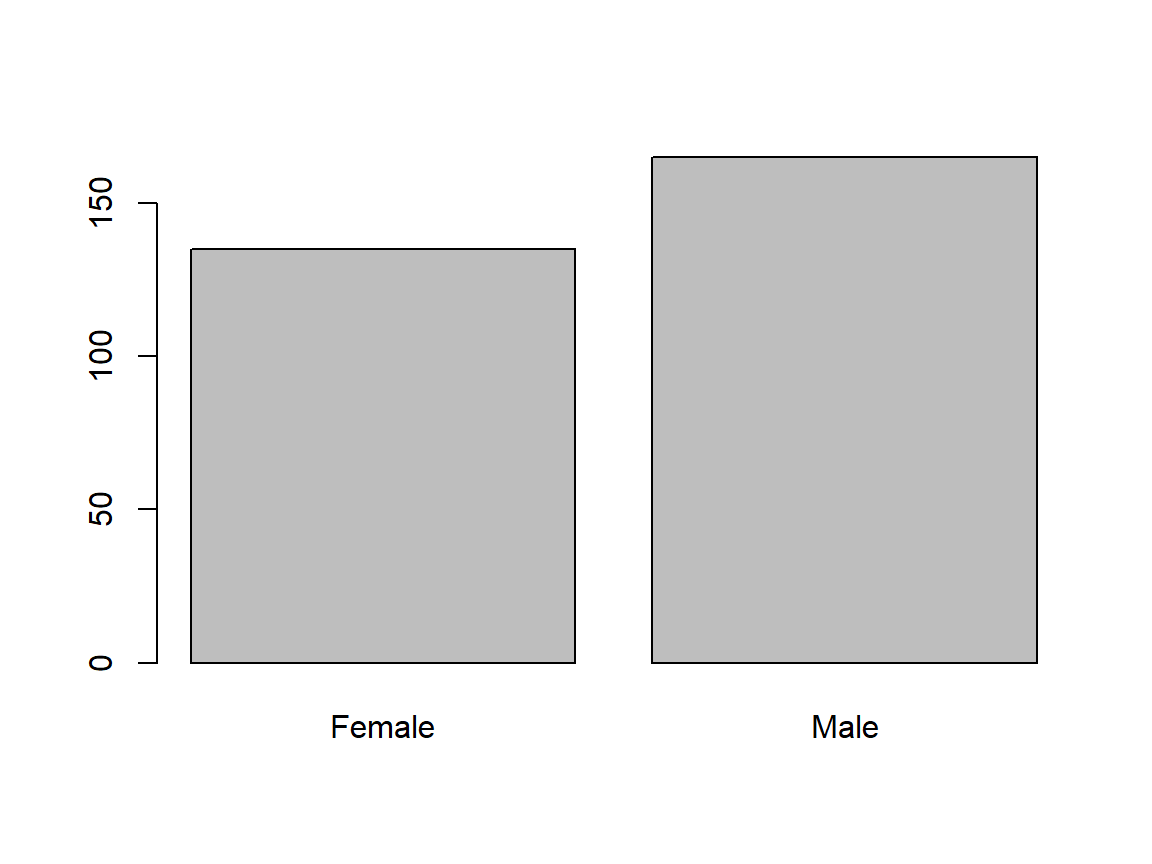
Sex

class(Sex)  # mode

## [1] "factor"

barplot(table(Sex))  # fitting?

Question	Answer
Mode?	factor
Which scale?	Binary
What’s implied?	Only two possible outcomes
Does data fit scale?	Yes

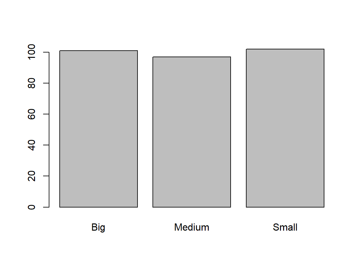
Size

class(Size)  # mode

## [1] "character"

barplot(table(Size))  # fitting?

Question	Answer
Mode?	character
Which scale?	Ordinal
What’s implied?	Categorical data that can be ordered
Does data fit scale?	Yes

Temperature

class(Temperature)  # mode

## [1] "numeric"

barplot(Temperature)  # fitting?

Question	Answer
Mode?	numeric
Which scale?	Interval/Discrete
What’s implied?	Continuous data with a non-absence point of origin
Does data fit scale?	Yes (the data is clearly recorded in degree Celsius)

Distributions

Length

plot(density(Length))  # distribution plot

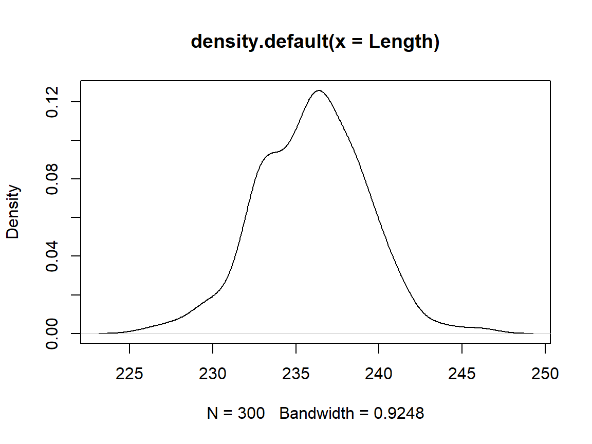
shapiro.test(Length)  # normality check

## 
## 	Shapiro-Wilk normality test
## 
## data:  Length
## W = 0.99496, p-value = 0.4331

The data is normal distributed.

Reproducing

plot(density(Reproducing))  # distribution

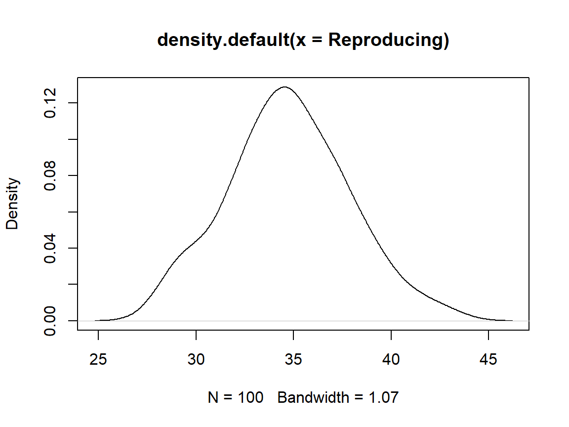
shapiro.test(Reproducing)  # normality check

## 
## 	Shapiro-Wilk normality test
## 
## data:  Reproducing
## W = 0.98444, p-value = 0.2889

The data is binomial distributed (i.e. “How many individuals manage to reproduce”) but looks normal distributed. The normal distribution doesn’t make sense here because it implies continuity whilst the data only comes in integers.

IndividualsPassingBy

plot(density(IndividualsPassingBy))  # distribution

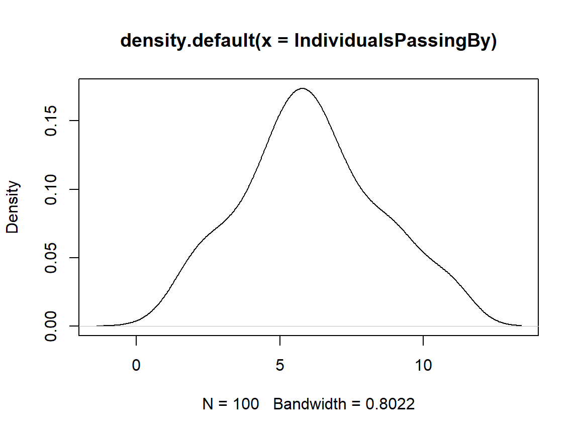
shapiro.test(IndividualsPassingBy)  # normality check

## 
## 	Shapiro-Wilk normality test
## 
## data:  IndividualsPassingBy
## W = 0.96905, p-value = 0.0187

The data is poisson distributed (i.e. “How many individuals pass by an observer in a given time frame?").

Depth

plot(density(Depth))  # distribution

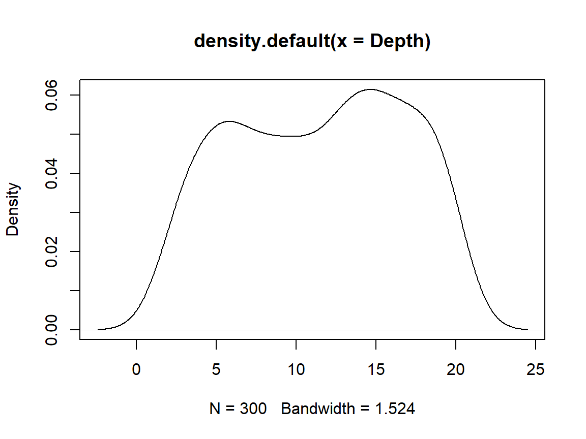
The data is uniform distributed. You don’t know this distribution class from the lectures and I only wanted to confuse you with this to show you that there’s much more out there than I can show in our lectures.