Hybrid Bayesian Networks
Material
- Hybrid Bayesian Networks
- Hybrid Bayesian Networks by Ariel Saffer (one of our study group members)
Exercises
These are answers and solutions to the exercises at the end of Part 3 in Bayesian Networks with Examples in R by M. Scutari and J.-B. Denis. Much of my inspiration for these solutions, where necessary, by consulting the solutions provided by the authors themselves as in the appendix.
R Environment
For today’s exercise, I load the following packages:
library(bnlearn)
library(rjags)
Scutari 3.1
Explain why it is logical to get a three-step function for the discretised approach in Figure 3.2.
Figure 3.2 shows this discretisation:
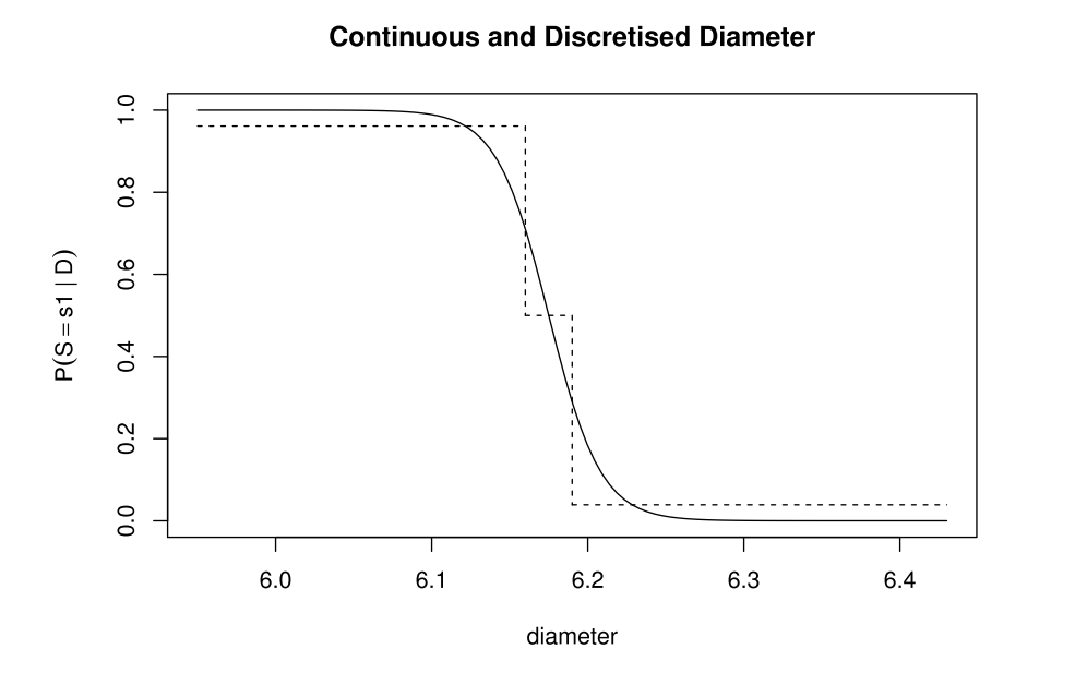
the reason we obtain a three-step function here is down to the intervals that were chosen to bin the continuous diametre data into discrete categories:
$$<6.16$$ $$[6.16; 6.19]$$ $$>6.19$$
Owing to these intervals, we fit all of our continuous data into three categories which mirror the three-step function portrayed in the above figure.
Scutari 3.2
Starting from the BUGS model in Section 3.1.1, write another BUGSmodel for the discretised model proposed in Section 3.1.2. The functions required for this task are described in the JAGS manual.
The model for the hybrid case (which we are to adapt to the discretised approach) reads as such:
model{
  csup ~ dcat(sp);
  cdiam ~ dnorm(mu[csup], 1/sigma^2);
}
To adapt it for discretised data, I simply change the outcome distribution for cdiam to also be categorical:
model{
  csup ~ dcat(sp);
  cdiam ~ dcat(Diams[, csup]);
}
where Diams is a matrix that contains probabilities for the different diameters (rows) for suppliers (columns).
Scutari 3.3
Let d = 6.0, 6.1, 6.2, 6.4.
- Using the BUGS model proposed in Section 3.1.1, write the
Rscript to estimate $P(S = s1 | D = d)$ for the continuous approach demonstrated in the same section.
I start by simply repeating the code in section 3.1.1:
sp <- c(0.5, 0.5)
mu <- c(6.1, 6.25)
sigma <- 0.05
From here, I take inspiration from the book in the later section on the crop model and write a sampling loop for which to retain samples. First, I create some objects to store data and outputs as well as do some housekeeping:
## house-keeping
set.seed(42) # there are random processes here

## object creation
diameters_vec <- c(6.0, 6.1, 6.2, 6.4)
prob_vec <- rep(NA, length(diameters_vec))
names(prob_vec) <- diameters_vec
Next, I greatly dislike the reliance on model files that the book insists on and so I register my JAGS model code as an active text connection in R:
jags_mod <- textConnection("model{
                           csup ~ dcat(sp);
                           cdiam ~ dnorm(mu[csup], 1/sigma^2);
                           }")
Finally, I am ready to estimate $P(S = s1 | D = d)$:
for (samp_iter in seq(length(diameters_vec))) {
  # create data list
  jags.data <- list(sp = sp, mu = mu, sigma = sigma, cdiam = diameters_vec[samp_iter])
  # compile model
  model <- jags.model(file = jags_mod, data = jags.data, quiet = TRUE)
  update(model, n.iter = 1e4)
  # sample model and retrieve vector of supplier identity (containing values 1 and 2)
  simu <- coda.samples(model = model, variable.names = "csup", n.iter = 2e4, thin = 20)[[1]]
  # compute probability of supplier 1
  prob_vec[samp_iter] <- sum(simu == 1) / length(simu)
}
prob_vec
##     6   6.1   6.2   6.4
## 1.000 0.982 0.197 0.000
- Using the BUGS model obtained in Exercise 3.2, write the
Rscript to estimate $P(S = s1 | D = d)$ for the discretised approach suggested in Section 3.1.2.
Again, I start by typing out important parameters from the book:
sp <- c(0.5, 0.5)
Diams <- matrix(c(0.88493, 0.07914, 0.03593, 0.03593, 0.07914, 0.88493), 3)
Diams
##         [,1]    [,2]
## [1,] 0.88493 0.03593
## [2,] 0.07914 0.07914
## [3,] 0.03593 0.88493
Once more, I perform housekeeping and object creation prior to sampling. This time, however, I create a probability matrix to store the probability of each rod diametre in each diametre class belonging to supplier 1:
## house-keeping
set.seed(42) # there are random processes here

## object creation
diameters_vec <- c(6.0, 6.1, 6.2, 6.4)
cdiam_vec <- 1:3
dimnames <- list(
  paste("cdiam", cdiam_vec, sep = "_"),
  diameters_vec
)
prob_mat <- matrix(rep(NA, 12), ncol = 4)
dimnames(prob_mat) <- dimnames
And there’s our model:
jags_mod <- textConnection("model{
                            csup ~ dcat(sp);
                            cdiam ~ dcat(Diams[, csup]);
                            }")
Finally, I am ready to estimate $P(S = s1 | D = d)$:
for (samp_iter in seq(length(cdiam_vec))) {
  # create data list
  jags.data <- list(sp = sp, Diams = Diams, cdiam = cdiam_vec[samp_iter])
  # compile model
  model <- jags.model(file = jags_mod, data = jags.data, quiet = TRUE)
  update(model, n.iter = 1e4)
  # sample model and retrieve vector of supplier identity (containing values 1 and 2)
  simu <- coda.samples(model = model, variable.names = "csup", n.iter = 2e4, thin = 20)[[1]]
  # compute probability of supplier 1
  prob_mat[samp_iter, ] <- sum(simu == 1) / length(simu)
}
prob_mat
##             6   6.1   6.2   6.4
## cdiam_1 0.966 0.966 0.966 0.966
## cdiam_2 0.490 0.490 0.490 0.490
## cdiam_3 0.035 0.035 0.035 0.035
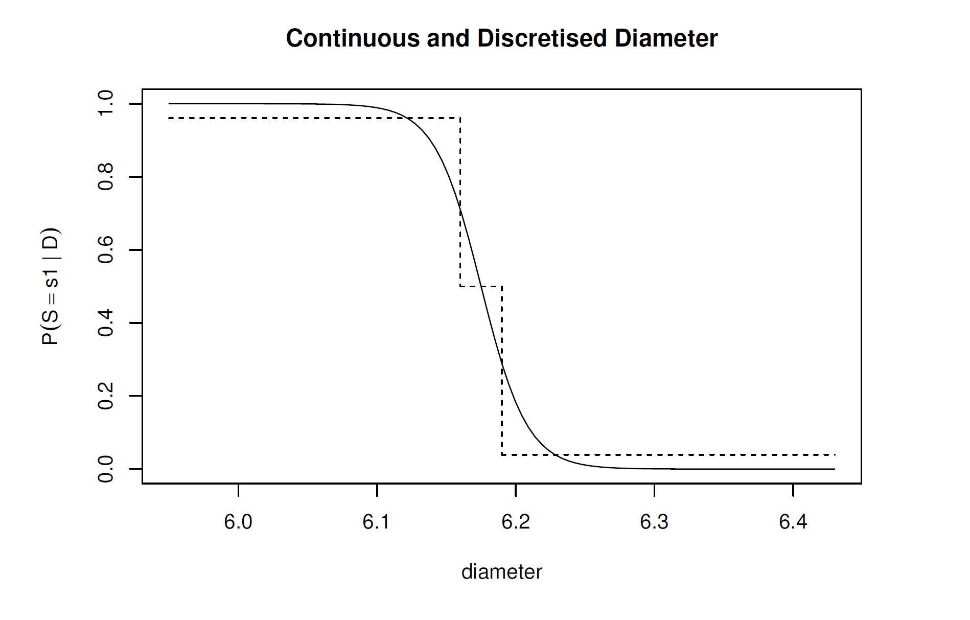
And check the results with Figure 3.2.
Looking at figure 3.2, I’d argue the above probabilities align with the figure:
Scutari 3.4
In Section 3.1.1, the probability that the supplier is
s1knowing that the diameter is 6.2 was estimated to be 0.1824 which is not identical to the value obtained with JAGS.
- Explain why the calculation with the
Rfunctiondnormis right and why the value 0.1824 is correct. Can you explain why the JAGS result is not exact? Propose a way to improve it.
Since either function relies on random processes, differences in seeds may explain the difference in inference. To improve the accuracy of the JAGS result, I would suggest increasing the sample size that led to its creation.
- Would this value be different if we modify the marginal distribution for the two suppliers?
Yes. Marginal distributions are essential to the Bayes' Theorem and a change thereof would necessitate a change in inference.
Scutari 3.5
Revisiting the discretisation in Section 3.1.2, compute the conditional probability tables for $ D | S $ and $ S | D $ when the interval boundaries are set to $ (6.10, 6.18) $ instead of $ (6.16, 6.19)$ . Compared to the results presented in Section 3.1.2, what is your conclusion?
Let’s start by repeating book code and updating the intervals to obtain $D | S$:
mu <- c(6.1, 6.25)
sigma <- 0.05
limits <- c(6.10, 6.18)
dsd <- matrix(
  c(
    diff(c(0, pnorm(limits, mu[1], sigma), 1)),
    diff(c(0, pnorm(limits, mu[2], sigma), 1))
  ),
  3, 2
)
dimnames(dsd) <- list(D = c("thin", "average", "thick"), S = c("s1", "s2"))
dsd
##          S
## D                 s1          s2
##   thin    0.50000000 0.001349898
##   average 0.44520071 0.079406761
##   thick   0.05479929 0.919243341
To obtain $ S | D $, we apply Bayes' Theorem:
jointd <- dsd / 2 # dive by 2 to get joint distribution over suppliers of which we have 2
mardd <- rowSums(jointd) # marginal distribution of diametre class irrespective of supplier
dds <- t(jointd / mardd) # find conditional probabilites
dds
##     D
## S           thin   average      thick
##   s1 0.997307473 0.8486359 0.05625964
##   s2 0.002692527 0.1513641 0.94374036
One of our new limits in in fact the mean diametre supplied by supplier 1. That is clearly not a helpful limit as it simply shifts probability to supplier 1.
Session Info
sessionInfo()
## R version 4.2.1 (2022-06-23 ucrt)
## Platform: x86_64-w64-mingw32/x64 (64-bit)
## Running under: Windows 10 x64 (build 19044)
##
## Matrix products: default
##
## locale:
## [1] LC_COLLATE=English_Germany.utf8  LC_CTYPE=English_Germany.utf8    LC_MONETARY=English_Germany.utf8 LC_NUMERIC=C                     LC_TIME=English_Germany.utf8
##
## attached base packages:
## [1] stats     graphics  grDevices utils     datasets  methods   base
##
## other attached packages:
## [1] rjags_4-13    coda_0.19-4   bnlearn_4.8.1
##
## loaded via a namespace (and not attached):
##  [1] bslib_0.4.0       compiler_4.2.1    pillar_1.8.1      jquerylib_0.1.4   R.methodsS3_1.8.2 R.utils_2.12.0    tools_4.2.1       digest_0.6.29     jsonlite_1.8.0    evaluate_0.16
## [11] lifecycle_1.0.2   R.cache_0.16.0    lattice_0.20-45   rlang_1.0.5       cli_3.3.0         rstudioapi_0.14   yaml_2.3.5        parallel_4.2.1    blogdown_1.13     xfun_0.33
## [21] fastmap_1.1.0     styler_1.8.0      stringr_1.4.1     knitr_1.40        vctrs_0.4.1       sass_0.4.2        grid_4.2.1        glue_1.6.2        R6_2.5.1          fansi_1.0.3
## [31] rmarkdown_2.16    bookdown_0.29     purrr_0.3.4       magrittr_2.0.3    htmltools_0.5.3   utf8_1.2.2        stringi_1.7.8     cachem_1.0.6      R.oo_1.25.0