(Bayesian) Networks & R
Material
Exercises
These are answers and solutions to the exercises at the end of chapter 1 in Bayesian Networks in R with Applications in Systems Biology by Radhakrishnan Nagarajan, Marco Scutari & Sophie Lèbre. Much of my inspiration for these solutions, where necessary, by consulting the solutions provided by the authors themselves as in the appendix.
Nagarajan 1.1
1.1. Consider a directed acyclic graph with n nodes.
(a) Show that at least one node must not have any incoming arc, i.e., the graph must contain at least one root node.
A graph without a root node violates the premise of acyclicity inherent to Bayesian Networks.
Assuming our graph is directed with G = (V, A), and assuming that there is no root node present, for any vertex $V_i$ that we chose of the set V, we can find a path that $V_i \rightarrow … \rightarrow V_n$ which spans all nodes in V. However, $V_n$ must have an outgoing arc ($V_n \rightarrow …$) which must connect to any of the nodes already on the path between $V_i$ and $V_n$ thereby incurring a loop or cycle.
(b) Show that such a graph can have at most n(n−1) arcs.
This can be explained as an iterative process. Starting with any node $V_1 \in \boldsymbol V$, not violating the prerequisite for acyclicity, $V_1$ may only contain $n-1$ outgoing arcs (an arc linking to itself would create a cycle). Continuing now to another node $V_2 \in \boldsymbol V$ and $V_2 \neq V_1$, this node may only contain $n-2$ outgoing arcs as any arc linking to itself or $V_1$ would introduce a cycle or loop.
Continuing this process to its logical conclusion of $V_n$, we can summarise the number of possible outgoing arcs thusly:
\begin{equation} A \leq (n-1) + (n-2) + … + (1) = \left( n\atop{2} \right) = \frac{n(n-1)}{2} \end{equation}
(c) Show that a path can span at most n−1 arcs.
Any arc contains two nodes - one tail and one head. Therefore, a path spanning n arcs would have to contain n+1 vertices, thus passing trough one vertex twice and introducing a cycle.
(d) Describe an algorithm to determine the topological ordering of the graph.
Two prominent examples are breadth-first (BF) and depth-first (DF) algorithms.
The former (BF) attempts to locate a node that satisfies a certain query conditions by exploring a graph from a root node and subsequently evaluating nodes which are equidistant to the root (at a distance of one arc). If none of these nodes satisfies the search criteria, the distance to root node is increased by an additional arc distance.
DF, on the other hand, starts at a root node and fully explores a randomly chosen path until either a node satisfying the search criteria is reached or the path has ended in which case a new path is explored starting at the root node.
Nagarajan 1.2
1.2. Consider the graphs shown in Fig. 1.1.
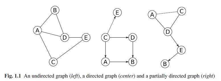
(a) Obtain the skeleton of the partially directed and directed graphs.
I start by loading the visNetwork R package. I chose this package simply because I like how it creates interactive visualisations - try it out! Click some of the vertices below or try and drag them around.
I also load additional html libraries with which I can include the thml outputs produced by visNetwork in this blog:
library(visNetwork)
library(htmlwidgets)
library(htmltools)
Next, I register the node set as well as the two arc sets we are working with:
V <- data.frame(
  id = c("A", "B", "C", "D", "E"),
  label = c("A", "B", "C", "D", "E")
)
A_directed <- data.frame(
  from = c("C", "C", "C", "D", "A"),
  to = c("E", "A", "D", "B", "B")
)
A_partial <- data.frame(
  from = c("E", "D", "A", "C", "C"),
  to = c("B", "E", "D", "D", "A")
)
Note that I still have to register a direction even for undirected edges.
Now, to visualise the skeletons, we simply plot the graphs without any edge directionality:
Click here for the plotting call of the skeleton of the directed graph:
## skeleton of directed graph
Nagara1.2aD <- visNetwork(
  nodes = V,
  edges = A_directed
) %>%
  visNodes(
    shape = "circle",
    font = list(size = 40, color = "white"),
    color = list(
      background = "darkgrey",
      border = "black",
      highlight = "orange"
    ),
    shadow = list(enabled = TRUE, size = 10)
  ) %>%
  visEdges(color = list(
    color = "green",
    highlight = "red"
  )) %>%
  visLayout(randomSeed = 42)
saveWidget(Nagara1.2aD, "Nagara1.2aD.html")
Click here for the plotting call of the skeleton of the partially directed graph:
## skeleton of partially directed graph
Nagara1.2aP <- visNetwork(
  nodes = V,
  edges = A_partial
) %>%
  visNodes(
    shape = "circle",
    font = list(size = 40, color = "white"),
    color = list(
      background = "darkgrey",
      border = "black",
      highlight = "orange"
    ),
    shadow = list(enabled = TRUE, size = 10)
  ) %>%
  visEdges(color = list(
    color = "green",
    highlight = "red"
  )) %>%
  visLayout(randomSeed = 42)

saveWidget(Nagara1.2aP, "Nagara1.2aP.html")
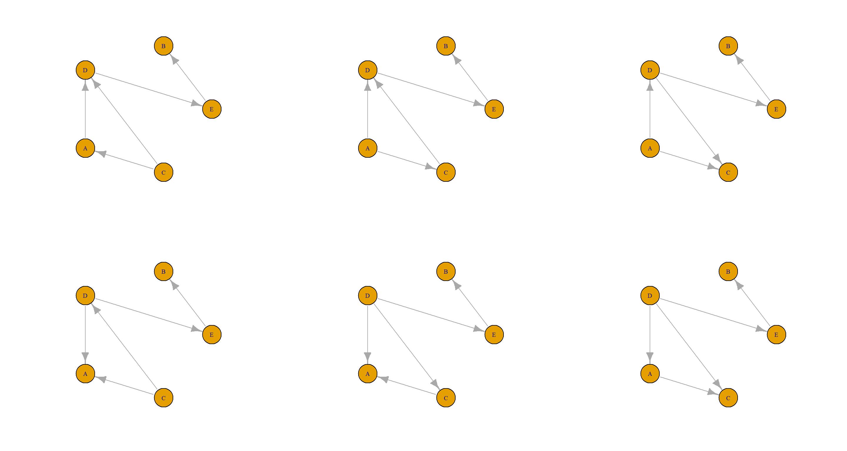
(b) Enumerate the acyclic graphs that can be obtained by orienting the undirected arcs of the partially directed graph.
Right. Sorting this out using visNetwork would be a royal pain. So I instead opt for using igraph for this exercise.
First, I load the necessary R package:
library(igraph)
Next, I consider the edge and node set of the partially directed graph:
V <- data.frame(id = c("A", "B", "C", "D", "E"))
A_partial <- data.frame(
  from = c("E", "D", "A", "C", "C"),
  to = c("B", "E", "D", "D", "A")
)
To enumerate all DAGs from these sets, I may only change the directions of the last three edges listed in my edge set.
Objectively, this exercise could be solved by simply thinking about the different constellations. However, I code for a living. One may argue that thinking is not necessarily in my wheelhouse (on may also claim the opposite). Hence, I will automate the procedure.
To do so, I will need to create all possible combinations of directions of currently undirected edges in the graph in question and check whether they create cycles or not.
To do so, I load the bnlearn package as it comes with an error message when trying to assign an arc set that introduces cycles. I also register a base graph consisting of only our vertex set:
library(bnlearn)
base_bn <- empty.graph(nodes = V$id)
Now, I simply loop over my three arcs in question and alternate which direction they are pointing. At the deepest level of this monstrosity, I am then assingning the final arcs to the base graph and only retain it if the cyclicity error has not been thrown:
A_iter <- A_partial
A_ls <- list()
counter <- 1
for (AD in 1:2) {
  A_iter[3, ] <- if (AD == 1) {
    A_partial[3, ]
  } else {
    rev(A_partial[3, ])
  }
  for (CD in 1:2) {
    A_iter[4, ] <- if (CD == 1) {
      A_partial[4, ]
    } else {
      rev(A_partial[4, ])
    }
    for (CA in 1:2) {
      A_iter[5, ] <- if (CA == 1) {
        A_partial[5, ]
      } else {
        rev(A_partial[5, ])
      }
      A_check <- tryCatch(
        {
          arcs(base_bn) <- A_iter
        },
        error = function(e) {
          "error"
        }
      )
      if (all(A_check != "error")) {
        A_ls[[counter]] <- base_bn
        counter <- counter + 1
      }
    }
  }
}
How many valid DAGs did this result in?
length(A_ls)
## [1] 6
Let’s plot these out and be done with it:
par(mfrow = c(2, 3))
for (plot_iter in A_ls) {
  dag_igraph <- graph_from_edgelist(arcs(plot_iter))
  plot(dag_igraph,
    layout = layout.circle,
    vertex.size = 30
  )
}
(c) List the arcs that can be reversed (i.e., turned in the opposite direction), one at a time, without introducing cycles in the directed graph.
All arcs of the directed graph can be reversed without introducing cycles.
Nagarajan 1.3
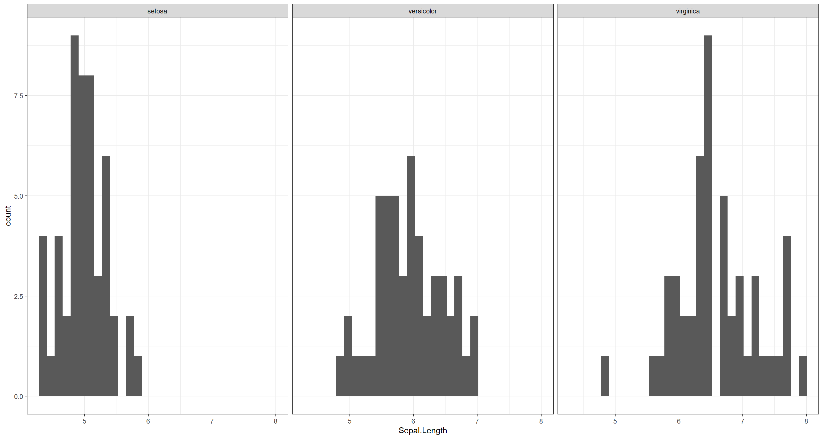
1.3. The (famous) iris data set reports the measurements in centimeters of the sepal length and width and the petal length and width for 50 flowers from each of 3 species of iris (“setosa,” “versicolor,” and “virginica”).
(a) Load the iris data set (it is included in the datasets package, which is part of the base R distribution and does not need to be loaded explicitly) and read its manual page.
data(iris)
?iris
(b) Investigate the structure of the data set.
str(iris)
## 'data.frame':	150 obs. of  5 variables:
##  $ Sepal.Length: num  5.1 4.9 4.7 4.6 5 5.4 4.6 5 4.4 4.9 ...
##  $ Sepal.Width : num  3.5 3 3.2 3.1 3.6 3.9 3.4 3.4 2.9 3.1 ...
##  $ Petal.Length: num  1.4 1.4 1.3 1.5 1.4 1.7 1.4 1.5 1.4 1.5 ...
##  $ Petal.Width : num  0.2 0.2 0.2 0.2 0.2 0.4 0.3 0.2 0.2 0.1 ...
##  $ Species     : Factor w/ 3 levels "setosa","versicolor",..: 1 1 1 1 1 1 1 1 1 1 ...
(c) Compare the sepal length among the three species by plotting histograms side by side.
library(ggplot2)
ggplot(iris, aes(x = Sepal.Length)) +
  geom_histogram() +
  facet_wrap(~Species) +
  theme_bw()
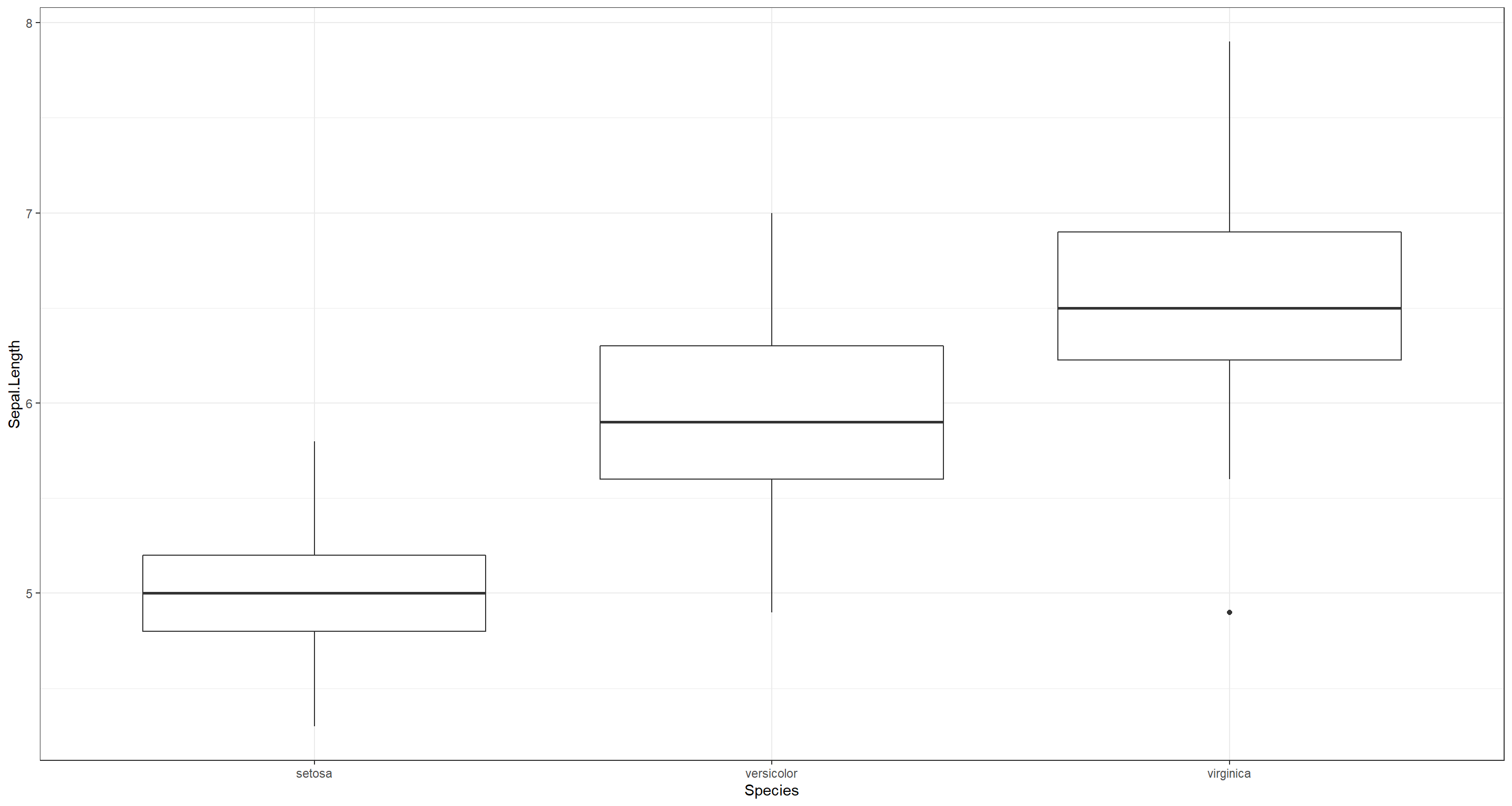
(d) Repeat the previous point using boxplots.
library(ggplot2)
ggplot(iris, aes(x = Species, y = Sepal.Length)) +
  geom_boxplot() +
  theme_bw()
Nagarajan 1.4
1.4. Consider again the iris data set from Exercise 1.3.
(a) Write the data frame holding iris data frame into a space-separated text file named “iris.txt,” and read it back into a second data frame called iris2.
write.table(iris, file = "iris.txt", row.names = FALSE)
iris2 <- read.table("iris.txt", header = TRUE)
(b) Check that iris and iris2 are identical.
identical(iris, iris2)
## [1] FALSE
Why are they not identical? That’s because iris stores Species as a factor. Information which is lost when writing to a .txt file. Let’s reformat this and check again:
iris2$Species <- factor(iris2$Species)
identical(iris, iris2)
## [1] TRUE
(c) Repeat the previous two steps with a file compressed with bzip2 named “iris.txt.bz2.”
bzfd <- bzfile("iris.txt.bz2", open = "w")
write.table(iris, file = bzfd, row.names = FALSE)
close(bzfd)
bzfd <- bzfile("iris.txt.bz2", open = "r")
iris2 <- read.table(bzfd, header = TRUE)
close(bzfd)
iris2$Species <- factor(iris2$Species)
identical(iris, iris2)
## [1] TRUE
(d) Save iris directly (e.g., without converting it to a text table) into a file called “iris.rda,” and read it back.
save(iris, file = "iris.rda")
load("iris.rda")
(e) List all R objects in the global environment and remove all of them apart from iris.
ls()
##  [1] "A_check"     "A_directed"  "A_iter"      "A_ls"        "A_partial"   "AD"          "base_bn"     "bzfd"        "CA"          "CD"          "counter"     "dag_igraph"  "iris"        "iris2"
## [15] "Nagara1.2aD" "Nagara1.2aP" "plot_iter"   "V"
l <- ls()
rm(list = l[l != "iris"])
(f) Exit the R saving the contents of the current session.
quit(save = "yes")
Nagarajan 1.5
1.5. Consider the gaussian.test data set included in bnlearn.
(a) Print the column names.
colnames(gaussian.test)
## [1] "A" "B" "C" "D" "E" "F" "G"
(b) Print the range and the quartiles of each variable.
## range
for (var in names(gaussian.test)) {
  print(range(gaussian.test[, var]))
}
## [1] -2.246520  4.847388
## [1] -10.09456  14.21538
## [1] -15.80996  32.44077
## [1] -9.043796 26.977326
## [1] -3.558768 11.494383
## [1] -1.170247 45.849594
## [1] -1.365823 12.409607
## quantiles
for (var in names(gaussian.test)) {
  print(quantile(gaussian.test[, var]))
}
##         0%        25%        50%        75%       100%
## -2.2465197  0.3240041  0.9836491  1.6896519  4.8473877
##           0%          25%          50%          75%         100%
## -10.09455807  -0.01751825   2.00025495   4.07692065  14.21537969
##         0%        25%        50%        75%       100%
## -15.809961   3.718150   8.056369  12.373614  32.440769
##        0%       25%       50%       75%      100%
## -9.043796  5.984274  8.994232 12.164417 26.977326
##        0%       25%       50%       75%      100%
## -3.558768  2.095676  3.508567  4.873497 11.494383
##        0%       25%       50%       75%      100%
## -1.170247 17.916175 21.982997 26.330886 45.849594
##        0%       25%       50%       75%      100%
## -1.365823  3.738940  5.028420  6.344179 12.409607
(c) Print all the observations for which A falls in the interval [3,4] and B in (−∞,−5]∪[10,∞).
TestA <- (gaussian.test[, "A"] >= 3) & (gaussian.test[, "A"] <= 4)
TestB <- (gaussian.test[, "B"] <= -4) | (gaussian.test[, "B"] >= 4)
gaussian.test[TestA & TestB, ]
##             A         B          C           D         E        F         G
## 134  3.000115  5.677259 19.6165914 13.90710134 1.2399546 29.66208 6.1184117
## 171  3.912097  5.000325 19.5261459 13.31373543 0.2807556 32.51754 7.3699037
## 954  3.735995  4.052434 18.1856087 12.09431457 3.7080579 26.97241 3.0517690
## 1034 3.317637  4.837303 18.1044125 13.32279487 2.9563555 28.40041 3.9876290
## 1042 3.372036  4.197395 17.6533233 12.52777893 4.8983597 31.08633 3.7283984
## 1078 3.157623  5.184670 19.0430676 13.89072391 3.2572347 37.08646 8.9429136
## 1127 3.141251  4.269507 17.1939411 12.42629251 2.6622288 29.53266 4.4132469
## 1237 3.031727  4.341881 17.6020776 12.43625964 2.7949498 27.74622 5.4084005
## 1755 3.052266  4.612071 18.1180989 13.19968750 5.6471997 27.78189 1.5129846
## 1819 3.290631  7.143942 22.6867359 16.14048867 4.8648686 37.51501 8.0241134
## 2030 3.289162  5.787095 20.0194963 14.52479092 5.2423368 37.46786 7.6643575
## 2153 3.037955  4.797399 17.1331929 13.58727751 2.7524554 31.84176 5.5202624
## 2179 3.114916  5.414628 19.3677155 14.14501162 3.4438786 31.06106 3.8799064
## 2576 3.458761  4.471637 18.1722539 13.36940122 2.3688318 23.60165 0.7689322
## 2865 3.140513  7.269383 22.5686681 16.86773531 4.0260061 36.17848 6.1028714
## 3035 3.476832  4.109519 17.0599625 11.55995675 4.4027366 29.83397 3.6381844
## 3133 3.667252  4.953129 19.6575484 13.31833594 5.0080665 31.78321 3.9031780
## 3434 3.418895  6.412021 21.8072576 15.48090391 5.6847825 29.41806 1.3941551
## 3481 3.050811  6.203747 21.1427355 15.39309314 4.2068982 33.79386 5.1348785
## 3573 3.612315  4.741220 18.4841065 13.08992732 5.4532191 31.22224 3.3986084
## 3695 3.284053  4.899003 17.7691812 13.73467842 4.5814578 39.96773 9.5808916
## 3893 3.070645  6.111989 20.6963754 15.34110860 2.0329921 29.92680 4.1352188
## 3999 3.493238  5.307218 19.1502279 14.10123450 4.8567953 35.69970 5.8485995
## 4144 3.045976  4.925688 18.8388604 13.28690773 7.3473994 34.12657 4.0527848
## 4164 3.624343  5.411443 20.3400016 13.35879870 7.4107565 32.20646 2.5717899
## 4220 3.133246  4.950543 17.9604182 13.91087282 4.2105519 30.01146 3.7960603
## 4229 3.119493  7.255816 22.4329800 16.59886045 2.4893039 33.62491 5.0819631
## 4258 3.777205  7.189762 23.9019969 16.75321069 4.0727603 37.66095 6.6653238
## 4671 3.455920 -4.198865  0.1452861 -0.27503006 1.9954874 16.60534 4.7261660
## 4703 3.301100 -4.109750  0.2244686 -0.07441052 6.2531813 23.58530 6.4627941
## 4739 3.010097  9.775164 28.1861733 20.54659992 5.1594216 40.50032 5.8467280
## 4779 3.215547  6.393758 20.7043512 15.59370075 3.2628127 33.35600 5.8151547
## 4866 3.873728 -4.257339  0.8213114 -0.31665717 0.2758219 14.94325 5.4011586
## 4987 3.058566  8.128704 24.9419446 18.56396890 5.8402279 35.29171 4.4032448
(d) Sample 50 rows without replacement.
I’m leaving out the output to save some space.
set.seed(42)
gaussian.test[sample(50, replace = FALSE), ]
(e) Draw a bootstrap sample (e.g., sample 5,000 observations with replacement) and compute the mean of each variable.
colMeans(gaussian.test[sample(5000, replace = TRUE), ])
##         A         B         C         D         E         F         G
##  1.007428  2.076592  8.157574  9.101292  3.532690 22.160643  4.998093
(f) Standardize each variable.
I’m leaving out the oputput to save some space.
scale(gaussian.test)
Nagarajan 1.6
1.6. Generate a data frame with 100 observations for the following variables:
(a) A categorical variable with two levels, low and high. The first 50 observations should be set to low, the others to high.
A <- factor(c(rep("low", 50), rep("high", 50)), levels = c("low", "high"))
(b) A categorical variable with two levels, good and bad, nested within the first variable, i.e., the first 25 observations should be set to good, the second 25 to bad, and so on.
nesting <- c(rep("good", 25), rep("bad", 25))
B <- factor(rep(nesting, 2), levels = c("good", "bad"))
(c) A continuous, numerical variable following a Gaussian distribution with mean 2 and variance 4 when the first variable is equal to low and with mean 4 and variance 1 if the first variable is equal to high. In addition, compute the standard deviation of the last variable for each configuration of the first two variables.
set.seed(42)
C <- c(rnorm(50, mean = 2, sd = 2), rnorm(50, mean = 4, sd = 1))
data <- data.frame(A = A, B = B, C = C)
aggregate(C ~ A + B, data = data, FUN = sd)
##      A    B         C
## 1  low good 2.6127294
## 2 high good 0.9712271
## 3  low  bad 1.8938398
## 4 high  bad 0.8943556