Dynamic Bayesian Networks

Material

Dynamic Bayesian Networks by Gregor Mathes (one of our study group members)

Exercises

These are answers and solutions to the exercises at the end of chapter 3 in Bayesian Networks in R with Applications in Systems Biology by by Radhakrishnan Nagarajan, Marco Scutari & Sophie Lèbre. Much of my inspiration for these solutions, where necessary, by consulting the solutions provided by the authors themselves as in the appendix.

`R` Environment

For today’s exercise, I load the following packages:

library(vars)
library(lars)
library(GeneNet)
library(G1DBN) # might have to run remotes::install_version("G1DBN", "3.1.1") first

Nagarajan 3.1

Consider the Canada data set from the vars package, which we analyzed in Sect. 3.5.1.

data(Canada)

Part A

Load the data set from the vars package and investigate its properties using the exploratory analysis techniques covered in Chap. 1.

str(Canada)

##  Time-Series [1:84, 1:4] from 1980 to 2001: 930 930 930 931 933 ...
##  - attr(*, "dimnames")=List of 2
##   ..$ : NULL
##   ..$ : chr [1:4] "e" "prod" "rw" "U"

summary(Canada)

##        e              prod             rw              U         
##  Min.   :928.6   Min.   :401.3   Min.   :386.1   Min.   : 6.700  
##  1st Qu.:935.4   1st Qu.:404.8   1st Qu.:423.9   1st Qu.: 7.782  
##  Median :946.0   Median :406.5   Median :444.4   Median : 9.450  
##  Mean   :944.3   Mean   :407.8   Mean   :440.8   Mean   : 9.321  
##  3rd Qu.:950.0   3rd Qu.:410.7   3rd Qu.:461.1   3rd Qu.:10.607  
##  Max.   :961.8   Max.   :418.0   Max.   :470.0   Max.   :12.770

Part B

Estimate a VAR(1) process for this data set.

(var1 <- VAR(Canada, p = 1, type = "const"))

## 
## VAR Estimation Results:
## ======================= 
## 
## Estimated coefficients for equation e: 
## ====================================== 
## Call:
## e = e.l1 + prod.l1 + rw.l1 + U.l1 + const 
## 
##          e.l1       prod.l1         rw.l1          U.l1         const 
##    1.17353629    0.14479389   -0.07904568    0.52438144 -192.56360758 
## 
## 
## Estimated coefficients for equation prod: 
## ========================================= 
## Call:
## prod = e.l1 + prod.l1 + rw.l1 + U.l1 + const 
## 
##         e.l1      prod.l1        rw.l1         U.l1        const 
##   0.08709510   1.01970070  -0.02629309   0.32299246 -81.55109611 
## 
## 
## Estimated coefficients for equation rw: 
## ======================================= 
## Call:
## rw = e.l1 + prod.l1 + rw.l1 + U.l1 + const 
## 
##        e.l1     prod.l1       rw.l1        U.l1       const 
##  0.06381103 -0.13551199  0.96872851 -0.19538479 11.61375726 
## 
## 
## Estimated coefficients for equation U: 
## ====================================== 
## Call:
## U = e.l1 + prod.l1 + rw.l1 + U.l1 + const 
## 
##         e.l1      prod.l1        rw.l1         U.l1        const 
##  -0.19293575  -0.08086896   0.07538624   0.47530976 186.80892410

Part C

Build the auto-regressive matrix $A$ and the constant matrix $B$ defining the VAR(1) model.

## base object creation
base_mat <- matrix(0, 4, 5)
colnames(base_mat) <- c("e", "prod", "rw", "U", "constant")
p <- 0.05
## object filling
pos <- which(coef(var1)$e[, "Pr(>|t|)"] < p)
base_mat[1, pos] <- coef(var1)$e[pos, "Estimate"]
pos <- which(coef(var1)$prod[, "Pr(>|t|)"] < p)
base_mat[2, pos] <- coef(var1)$prod[pos, "Estimate"]
pos <- which(coef(var1)$rw[, "Pr(>|t|)"] < p)
base_mat[3, pos] <- coef(var1)$rw[pos, "Estimate"]
pos <- which(coef(var1)$U[, "Pr(>|t|)"] < p)
base_mat[4, pos] <- coef(var1)$U[pos, "Estimate"]
## final objects
(A <- base_mat[, 1:4])

##               e        prod          rw         U
## [1,]  1.1735363  0.14479389 -0.07904568 0.5243814
## [2,]  0.0000000  1.01970070  0.00000000 0.0000000
## [3,]  0.0000000 -0.13551199  0.96872851 0.0000000
## [4,] -0.1929358 -0.08086896  0.07538624 0.4753098

(B <- base_mat[, 5])

## [1] -192.5636    0.0000    0.0000  186.8089

Part D

Compare the results with the LASSO matrix when estimating the L1-penalty with cross-validation.

## data preparation
data_df <- Canada[-nrow(Canada), ] # remove last row of data
## Lasso
Lasso_ls <- lapply(colnames(Canada), function(gene) {
  y <- Canada[-1, gene] # remove first row of data, and select only target gene
  lars(y = y, x = data_df, type = "lasso") # LASSO matrix
})
## Cross-validation
CV_ls <- lapply(1:ncol(Canada), function(gene) {
  y <- Canada[-1, gene] # remove first row of data, and select only target gene
  lasso.cv <- cv.lars(y = y, x = data_df, mode = "fraction")
  frac <- lasso.cv$index[which.min(lasso.cv$cv)]
  predict(Lasso_ls[[gene]], s = frac, type = "coef", mode = "fraction")
})
## output
rbind(
  CV_ls[[1]]$coefficients,
  CV_ls[[2]]$coefficients,
  CV_ls[[3]]$coefficients,
  CV_ls[[4]]$coefficients
)

##                e        prod           rw          U
## [1,]  1.17353629  0.14479389 -0.079045685  0.5243814
## [2,]  0.02570001  1.02314558 -0.004878295  0.1994059
## [3,]  0.09749788 -0.11991692  0.954389035 -0.1023845
## [4,] -0.17604953 -0.08192783  0.069502065  0.5086115

And for comparison the previously identified $A$:

##               e        prod          rw         U
## [1,]  1.1735363  0.14479389 -0.07904568 0.5243814
## [2,]  0.0000000  1.01970070  0.00000000 0.0000000
## [3,]  0.0000000 -0.13551199  0.96872851 0.0000000
## [4,] -0.1929358 -0.08086896  0.07538624 0.4753098

Part E

What can you conclude?

The whole point of LASSO, as far as I understand it, is to shrink parameter estimates towards 0 often times reaching 0 exactly. In the above this has not happened for many parameters, but is the case with the estimation provided by vars. I assume this might be because there just aren’t enough variables and/or observations in time.

Nagarajan 3.2

Consider the arth800 data set from the GeneNet package, which we analyzed in Sects. 3.5.2 and 3.5.3.

data(arth800)
data(arth800.expr)

Part A

Load the data set from the GeneNet package. The time series expression of the 800 genes is included in a data set called arth800.expr. Investigate its properties using the exploratory analysis techniques covered in Chap. 1.

str(arth800.expr)

##  'longitudinal' num [1:22, 1:800] 10.04 10.11 9.77 10.06 10.02 ...
##  - attr(*, "dimnames")=List of 2
##   ..$ : chr [1:22] "0-1" "0-2" "1-1" "1-2" ...
##   ..$ : chr [1:800] "AFFX-Athal-GAPDH_3_s_at" "AFFX-Athal-Actin_3_f_at" "267612_at" "267520_at" ...
##  - attr(*, "time")= num [1:11] 0 1 2 4 8 12 13 14 16 20 ...
##  - attr(*, "repeats")= num [1:11] 2 2 2 2 2 2 2 2 2 2 ...

summary(arth800.expr)

## Longitudinal data:
##  800 variables measured at 11 different time points
##  Total number of measurements per variable: 22 
##  Repeated measurements: yes 
## 
##  To obtain the measurement design call 'get.time.repeats()'.

Part B

For this practical exercise, we will work on a subset of variables (one for each gene) having a large variance. Compute the variance of each of the 800 variables, plot the various variance values in decreasing order, and create a data set with the variables greater than 2.

## variance calculation
variance <- diag(var(arth800.expr))
## plotting
plot(sort(variance, decreasing = TRUE), type = "l", ylab = "Variance")
abline(h = 2, lty = 2)

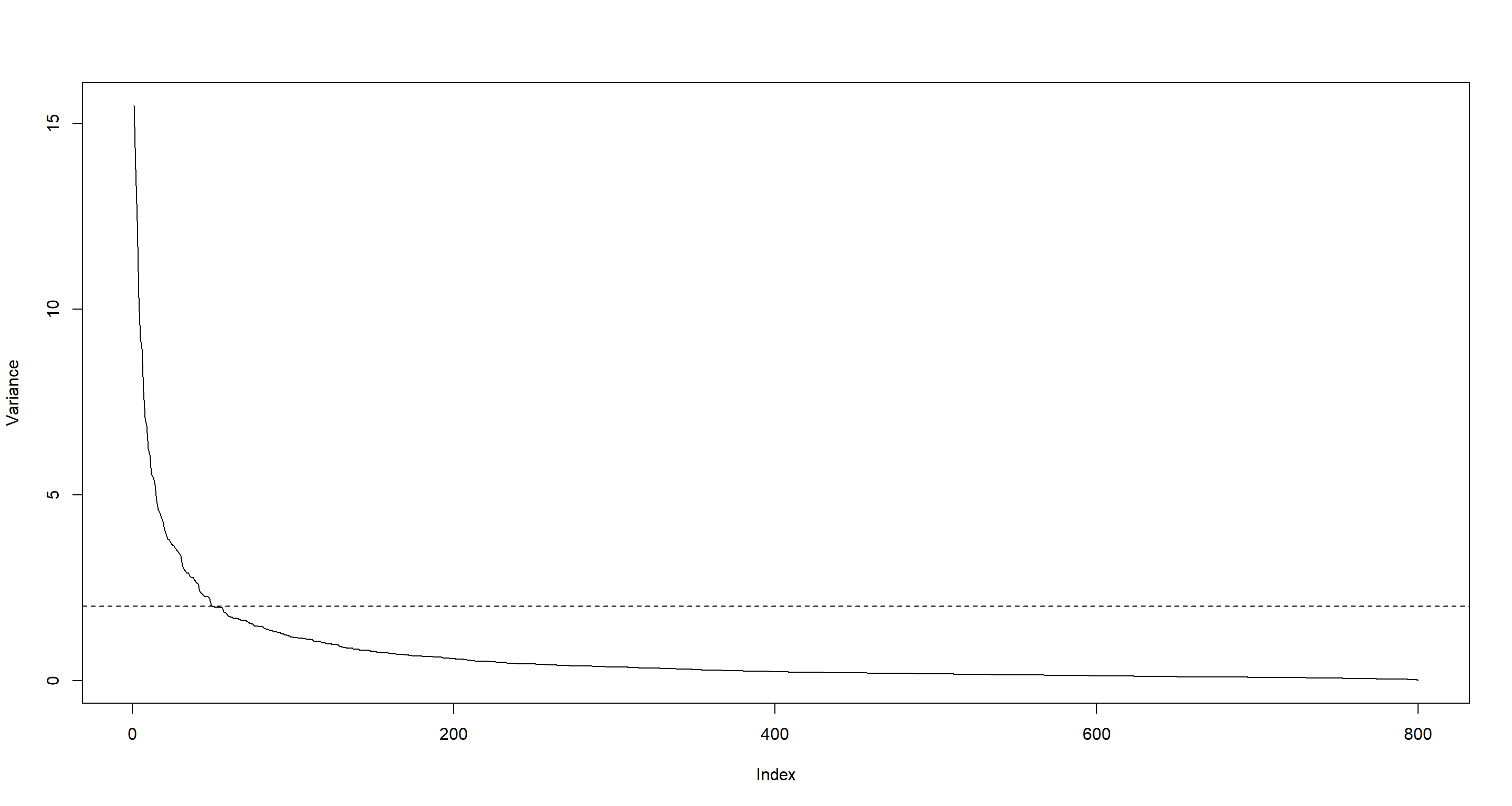
## variables with variances greater than 2
dataVar2 <- arth800.expr[, which(variance > 2)]
dim(dataVar2)

## [1] 22 49

Part C

Can you fit a VAR process with a usual approach from this data set?

I don’t think so. There are more variables (genes) than there are samples (time steps):

dim(dataVar2)

## [1] 22 49

Part D

Which alternative approaches can be used to fit a VAR process from this data set?

The chapter discusses these alternatives:

LASSO
James-Stein Shrinkage
Low-order conditional dependency approximation

Part E

Estimate a dynamic Bayesian network with each of the alternative approaches presented in this chapter.

First, I prepare the data by re-ordering them:

## make the data sequential for both repetitions
dataVar2seq <- dataVar2[c(seq(1, 22, by = 2), seq(2, 22, by = 2)), ]

LASSO with the lars package:

x <- dataVar2seq[-c(21:22), ] # remove final rows (end of sequences)
Lasso_ls <- lapply(colnames(dataVar2seq), function(gene) {
  y <- dataVar2seq[-(1:2), gene]
  lars(y = y, x = x, type = "lasso")
})
CV_ls <- lapply(1:ncol(dataVar2seq), function(gene) {
  y <- dataVar2seq[-(1:2), gene]
  lasso.cv <- cv.lars(y = y, x = x, mode = "fraction", plot.it = FALSE)
  frac <- lasso.cv$index[which.min(lasso.cv$cv)]
  predict(Lasso_ls[[gene]], s = frac, type = "coef", mode = "fraction")
})
Lasso_mat <- matrix(0, dim(dataVar2seq)[2], dim(dataVar2seq)[2])
for (i in 1:dim(Lasso_mat)[1]) {
  Lasso_mat[i, ] <- CV_ls[i][[1]]$coefficients
}
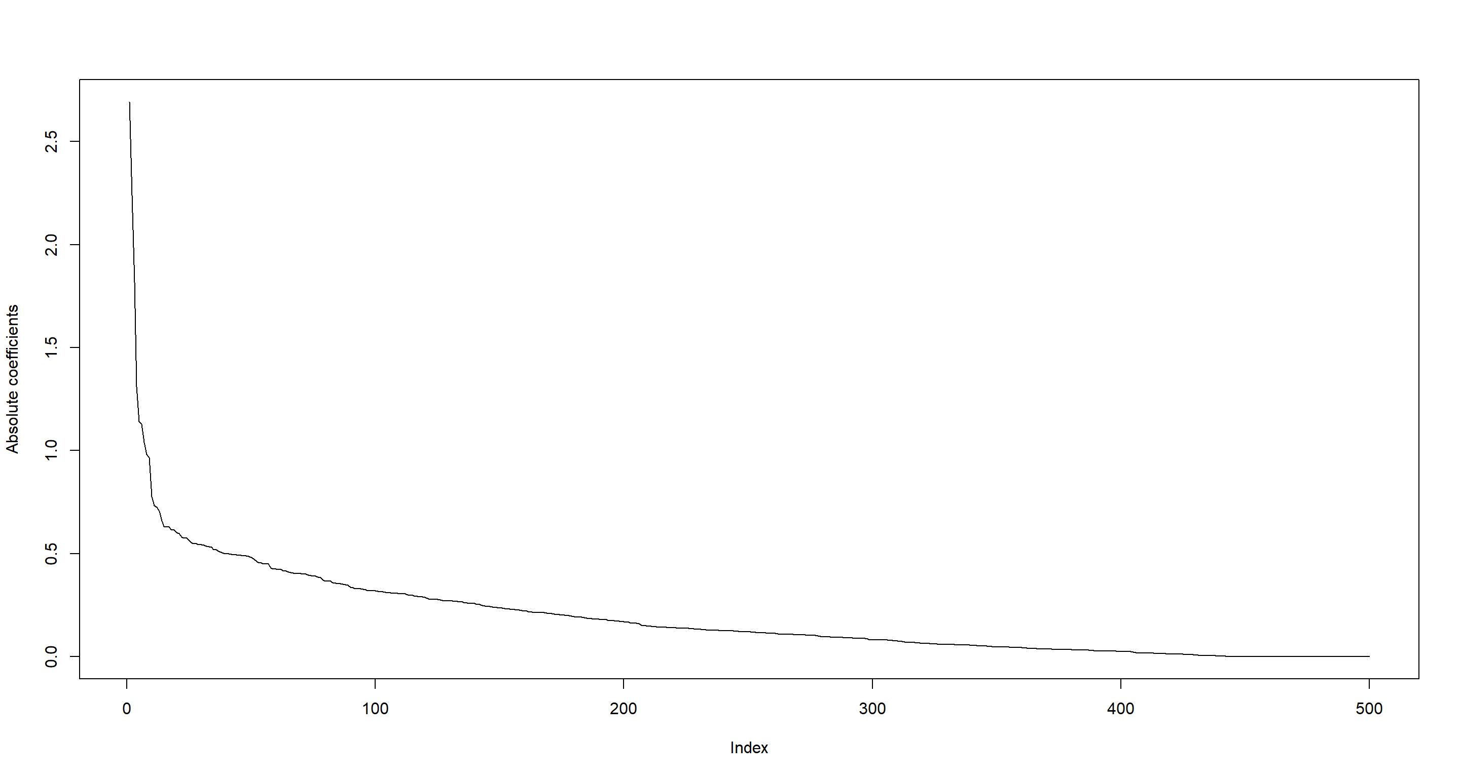
sum(Lasso_mat != 0) # number of arcs

## [1] 456

plot(sort(abs(Lasso_mat), decr = TRUE)[1:500], type = "l", ylab = "Absolute coefficients")

James-Stein shrinkage with the GeneNet package:

DBNGeneNet <- ggm.estimate.pcor(dataVar2, method = "dynamic")

## Estimating optimal shrinkage intensity lambda (correlation matrix): 0.0539

DBNGeneNet.edges <- network.test.edges(DBNGeneNet) # p-values, q-values and posterior probabilities for each potential arc

## Estimate (local) false discovery rates (partial correlations):
## Step 1... determine cutoff point
## Step 2... estimate parameters of null distribution and eta0
## Step 3... compute p-values and estimate empirical PDF/CDF
## Step 4... compute q-values and local fdr
## Step 5... prepare for plotting

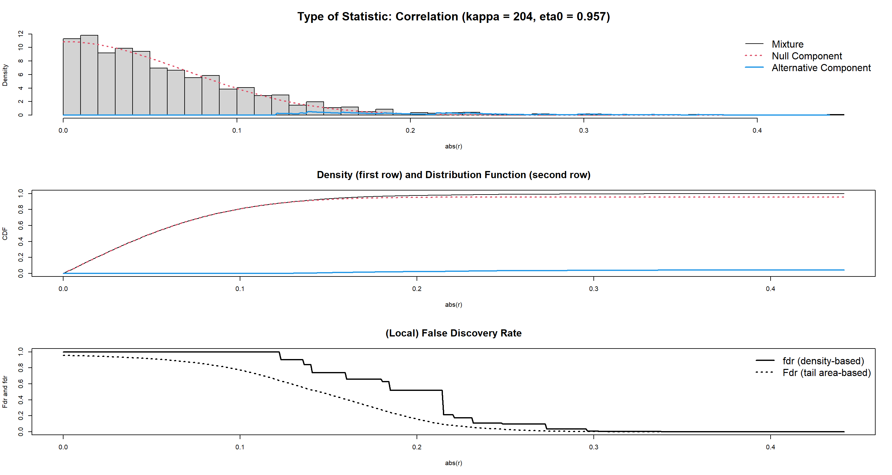
plot(DBNGeneNet.edges[, "prob"], type = "l") # arcs probability by decreasing order

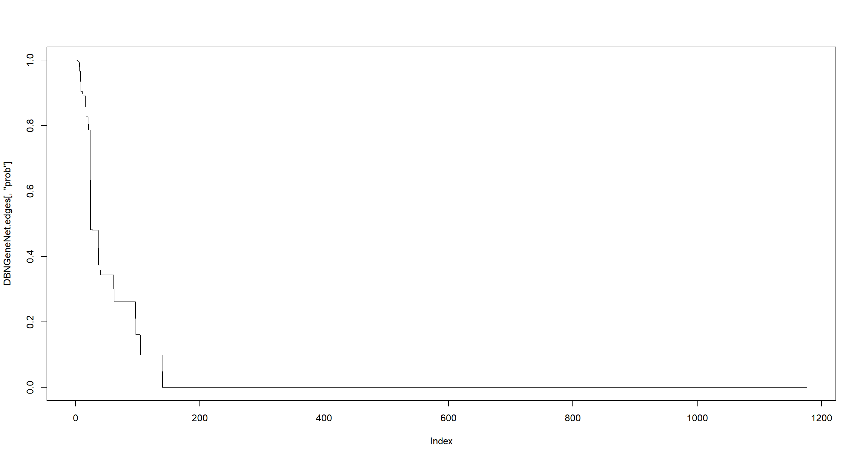
sum(DBNGeneNet.edges$prob > 0.95) # arcs with prob > 0.95

## [1] 8

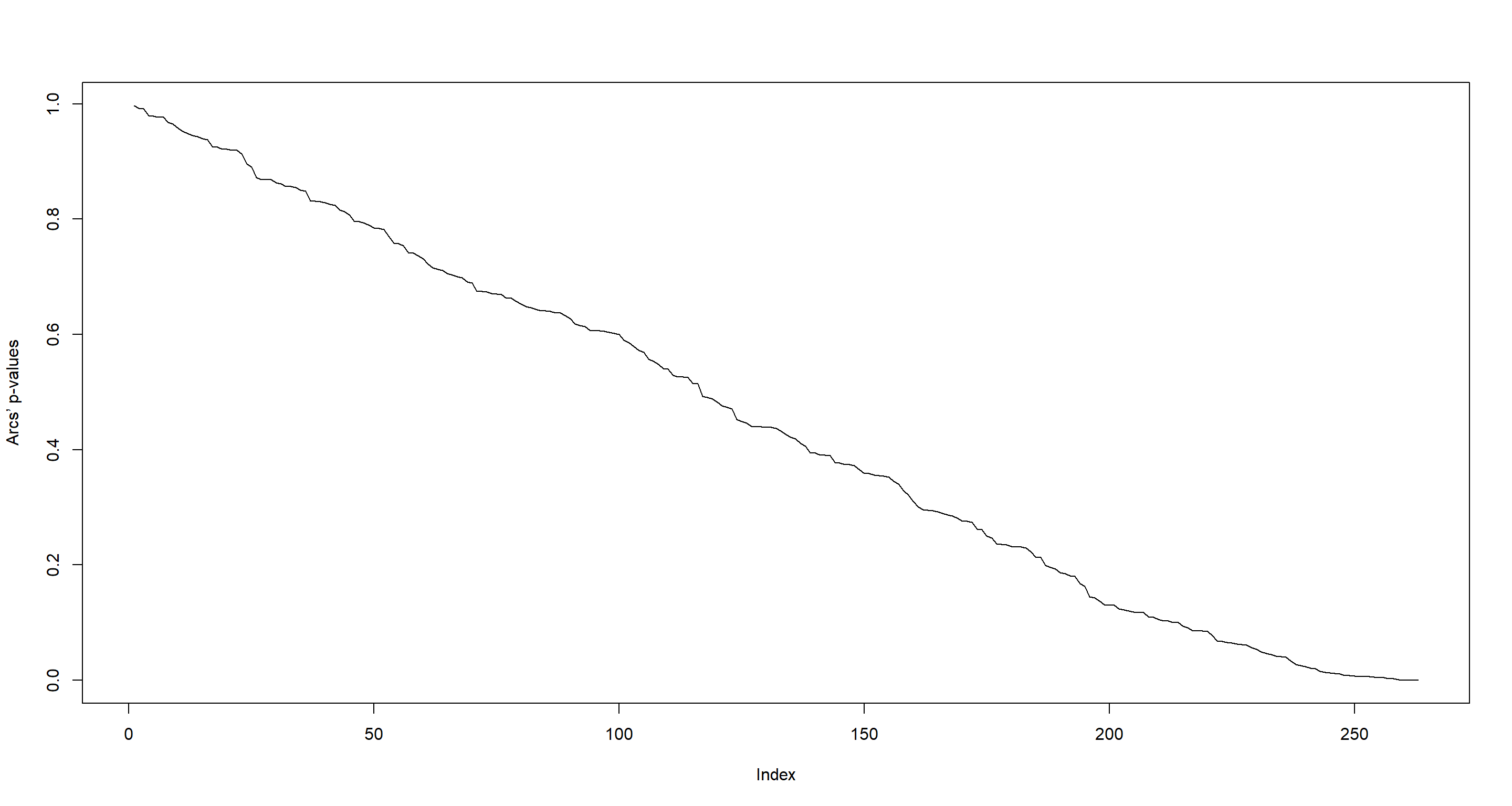
First-order conditional dependency with the G1DBN package:

G1DB_BN <- DBNScoreStep1(dataVar2seq, method = "ls")

## Treating 49 vertices:
## 10% 20% 30% 40% 50% 60% 70% 80% 90% 100%

G1DB_BN <- DBNScoreStep2(G1DB_BN$S1ls, dataVar2seq, method = "ls", alpha1 = 0.5)
plot(sort(G1DB_BN, decreasing = TRUE), type = "l", ylab = "Arcs’ p-values")

Nagarajan 3.3

Consider the dimension reduction approaches used in the previous exercise and the arth800 data set from the GeneNet package.

data(arth800)
data(arth800.expr)

Part A

For a comparative analysis of the different approaches, select the top 50 arcs for each approach (function BuildEdges from the G1DBN package can be used to that end).

LASSO

lasso_tresh <- mean(sort(abs(Lasso_mat), decreasing = TRUE)[50:51]) # Lasso_mat from exercise 3.2
lasso_50 <- BuildEdges(score = -abs(Lasso_mat), threshold = -lasso_tresh)

James-Stein shrinkage with the GeneNet package:

DBNGeneNet_50 <- cbind(DBNGeneNet.edges[1:50, "node1"], DBNGeneNet.edges[1:50, "node2"])

First-order conditional dependency with the G1DBN package:

G1DBN_tresh <- mean(sort(G1DB_BN)[50:51])
G1DBN.edges <- BuildEdges(score = G1DB_BN, threshold = G1DBN_tresh, prec = 3)

Part B

Plot the four inferred networks with the function plot from package G1DBN.

Four inferred networks? I assume the exercise so far wanted me to also analyse the data using the LASSO approach with the SIMoNe (simone) package. I will skip over that one and continue with the three I have:

par(mfrow = c(1, 3))

## LASSO
LASSO_plot <- graph.edgelist(cbind(lasso_50[, 1], lasso_50[, 2]))
Lasso_layout <- layout.fruchterman.reingold(LASSO_plot)
plot(LASSO_plot,
  layout = Lasso_layout,
  edge.arrow.size = 0.5, vertex.size = 10,
  main = "LASSO"
)

## James-Stein
DBN_plot <- graph.edgelist(DBNGeneNet_50)
# DBN_layout <- layout.fruchterman.reingold(DBN_plot)
plot(DBN_plot,
  layout = Lasso_layout,
  edge.arrow.size = 0.5, vertex.size = 10,
  main = "GeneNet"
)

## First-order conditional
G1DBN_plot <- graph.edgelist(cbind(G1DBN.edges[, 1], G1DBN.edges[, 2]))
# G1DBN_layout = layout.fruchterman.reingold(G1DBN_plot)
plot(G1DBN_plot,
  layout = Lasso_layout,
  edge.arrow.size = 0.5, vertex.size = 10,
  main = "G1DBN"
)

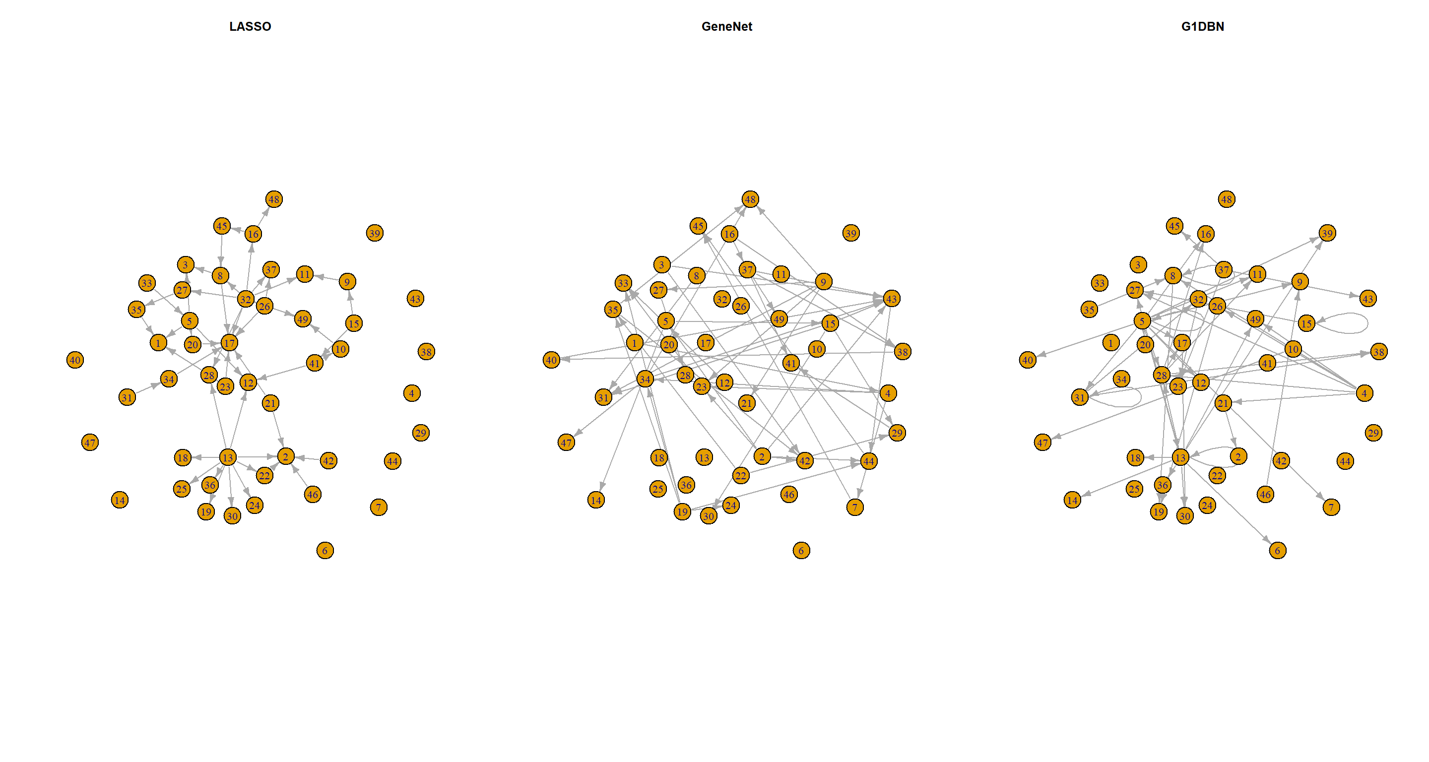
Part C

How many arcs are common to the four inferred networks?

## extract edges
LASSO_el <- as_edgelist(LASSO_plot)
DBN_el <- as_edgelist(DBN_plot)
G1DBN_el <- as_edgelist(G1DBN_plot)

## number of repeated edges in pairwise comparisons
sum(duplicated(rbind(LASSO_el, DBN_el)))

## [1] 0

sum(duplicated(rbind(LASSO_el, G1DBN_el)))

## [1] 6

sum(duplicated(rbind(DBN_el, G1DBN_el)))

## [1] 1

### all at once
sum(duplicated(rbind(LASSO_el, DBN_el, G1DBN_el)))

## [1] 7

Part D

Are the top 50 arcs of each inferred network similar? What can you conclude?

No, they are not. I can conclude that different dimension reductions produce different DAG structures.

Session Info

sessionInfo()

## R version 4.2.1 (2022-06-23 ucrt)
## Platform: x86_64-w64-mingw32/x64 (64-bit)
## Running under: Windows 10 x64 (build 19044)
## 
## Matrix products: default
## 
## locale:
## [1] LC_COLLATE=English_Germany.utf8  LC_CTYPE=English_Germany.utf8    LC_MONETARY=English_Germany.utf8 LC_NUMERIC=C                     LC_TIME=English_Germany.utf8    
## 
## attached base packages:
## [1] stats     graphics  grDevices utils     datasets  methods   base     
## 
## other attached packages:
##  [1] G1DBN_3.1.1         igraph_1.3.4        GeneNet_1.2.16      fdrtool_1.2.17      longitudinal_1.1.13 corpcor_1.6.10      lars_1.3            vars_1.5-6          lmtest_0.9-40      
## [10] urca_1.3-3          strucchange_1.5-3   sandwich_3.0-2      zoo_1.8-10          MASS_7.3-58.1      
## 
## loaded via a namespace (and not attached):
##  [1] highr_0.9         bslib_0.4.0       compiler_4.2.1    jquerylib_0.1.4   R.methodsS3_1.8.2 R.utils_2.12.0    tools_4.2.1       digest_0.6.29     jsonlite_1.8.0    evaluate_0.16    
## [11] nlme_3.1-159      R.cache_0.16.0    lattice_0.20-45   pkgconfig_2.0.3   rlang_1.0.5       cli_3.3.0         rstudioapi_0.14   yaml_2.3.5        blogdown_1.13     xfun_0.33        
## [21] fastmap_1.1.0     styler_1.8.0      stringr_1.4.1     knitr_1.40        vctrs_0.4.1       sass_0.4.2        grid_4.2.1        R6_2.5.1          rmarkdown_2.16    bookdown_0.29    
## [31] purrr_0.3.4       magrittr_2.0.3    htmltools_0.5.3   stringi_1.7.8     cachem_1.0.6      R.oo_1.25.0

Last updated on Nov 1, 2022

Dynamic Bayesian Networks

Material

Exercises

R Environment

Nagarajan 3.1

Part A

Part B

Part C

Part D

Part E

Nagarajan 3.2

Part A

Part B

Part C

Part D

Part E

Nagarajan 3.3

Part A

Part B

Part C

Part D

Session Info

Related

`R` Environment