Model Selection
Theory
These are exercises and solutions meant as a compendium to my talk on Model Selection and Model Building.
I have prepared some I have prepared some Lecture Slides for this session. For a more mathematical look at these concepts, I cannot recommend enough Eduardo García Portugués' blog.
R Environment
For this exercise, we will need the following packages:
install.load.package <- function(x) {
  if (!require(x, character.only = TRUE)) {
    install.packages(x, repos = "http://cran.us.r-project.org")
  }
  require(x, character.only = TRUE)
}
package_vec <- c(
  "ggplot2", # for visualisation
  "leaflet", # for maps
  "splitstackshape", # for stratified sampling
  "caret", # for cross-validation exercises
  "boot", # for bootstrap parameter estimates
  "tidyr", # for reshaping data frames
  "tidybayes", # for visualisation of bootstrap estimates
  "pROC", # for ROC-curves
  "olsrr", # for subset selection
  "MASS", # for stepwise subset selection
  "nlme", # for mixed effect models
  "mclust", # for k-means clustering,
  "randomForest", # for randomForest classifier
  "lmeresampler" # for validation of lmer models
)
sapply(package_vec, install.load.package)
##         ggplot2         leaflet splitstackshape           caret            boot           tidyr       tidybayes            pROC           olsrr            MASS            nlme          mclust
##            TRUE            TRUE            TRUE            TRUE            TRUE            TRUE            TRUE            TRUE            TRUE            TRUE            TRUE            TRUE
##    randomForest    lmeresampler
##            TRUE            TRUE
Using the above function is way more sophisticated than the usual install.packages() & library() approach since it automatically detects which packages require installing and only install these thus not overwriting already installed packages.
Our Resarch Project
Today, we are looking at a big (and entirely fictional) data base of the common house sparrow (Passer domesticus). In particular, we are interested in the Evolution of Passer domesticus in Response to Climate Change which was previously explained here.
The Data
I have created a large data set for this exercise which is available here and we previously cleaned up so that is now usable here.
Reading the Data into R
Let’s start by reading the data into R and taking an initial look at it:
Sparrows_df <- readRDS(file.path("Data", "SparrowDataClimate.rds"))
head(Sparrows_df)
##   Index Latitude Longitude     Climate Population.Status Weight Height Wing.Chord Colour    Sex Nesting.Site Nesting.Height Number.of.Eggs Egg.Weight Flock Home.Range Predator.Presence Predator.Type
## 1    SI       60       100 Continental            Native  34.05  12.87       6.67  Brown   Male         <NA>             NA             NA         NA     B      Large               Yes         Avian
## 2    SI       60       100 Continental            Native  34.86  13.68       6.79   Grey   Male         <NA>             NA             NA         NA     B      Large               Yes         Avian
## 3    SI       60       100 Continental            Native  32.34  12.66       6.64  Black Female        Shrub          35.60              1       3.21     C      Large               Yes         Avian
## 4    SI       60       100 Continental            Native  34.78  15.09       7.00  Brown Female        Shrub          47.75              0         NA     E      Large               Yes         Avian
## 5    SI       60       100 Continental            Native  35.01  13.82       6.81   Grey   Male         <NA>             NA             NA         NA     B      Large               Yes         Avian
## 6    SI       60       100 Continental            Native  32.36  12.67       6.64  Brown Female        Shrub          32.47              1       3.17     E      Large               Yes         Avian
##       TAvg      TSD
## 1 269.9596 15.71819
## 2 269.9596 15.71819
## 3 269.9596 15.71819
## 4 269.9596 15.71819
## 5 269.9596 15.71819
## 6 269.9596 15.71819
Hypotheses
Let’s remember our hypotheses:
- Sparrow Morphology is determined by:
A. Climate Conditions with sparrows in stable, warm environments fairing better than those in colder, less stable ones.
B. Competition with sparrows in small flocks doing better than those in big flocks.
C. Predation with sparrows under pressure of predation doing worse than those without. - Sites accurately represent sparrow morphology. This may mean:
A. Population status as inferred through morphology.
B. Site index as inferred through morphology.
C. Climate as inferred through morphology.
We have already built some models for these here and here.
Candidate Models
Before we can get started on model selection and validation, we need some actual models. Let’s create some. Since the data set contains three variables pertaining to sparrow morphology (i.e. Weight, Height, Wing.Chord) and I don’t want this exercise to spiral out of control with models that account for more than one response variable, we need to settle on one as our response variable in the first hypothesis. I am going with Weight.
Additionally, because I am under a bit of time pressure in creating this material, I forego all checking of assumptions on any of the following candidate models as the goal with this material is model selection/validation and not model assumption checking.
Continuous Models
load(file = file.path("Data", "H1_Models.RData"))
This just loaded three objects into R:
H1_ModelSparrows_ls- a list of candidate models built for the entireSparrow_dfdata setSparrows_df- the data frame used to build the global candidate modelsH1_ModelCNA_ls- a list of candidate models built just for three coastal sites across Central and North AmericaCentralNorthAm_df- the data frame used to build the candidate model for Central and North America
Global Models
Global regression models include:
sapply(H1_ModelSparrows_ls, "[[", "call")
## $Null
## lm(formula = Weight ~ 1, data = Sparrows_df)
##
## $Comp_Flock.Size
## lm(formula = Weight ~ Flock.Size, data = Sparrows_df)
##
## $Comp_Full
## lm(formula = Weight ~ Home.Range * Flock.Size, data = Sparrows_df)
##
## $Full
## lm(formula = Weight ~ Climate + TAvg + TSD + Home.Range * Flock.Size +
##     Predator.Type, data = Sparrows_df)
##
## $Mixed_Full
## lme.formula(fixed = Weight ~ Predator.Type + Flock.Size * Home.Range +
##     TAvg + TSD, data = Sparrows_df, random = list(Population.Status = ~1))
Local Models
Local regression models for the region of Central/North America include:
sapply(H1_ModelCNA_ls, "[[", "call")
## $Null
## lm(formula = Weight ~ 1, data = CentralNorthAm_df)
##
## $Clim_TAvg
## lm(formula = Weight ~ TAvg, data = CentralNorthAm_df)
##
## $Clim_TSD
## lm(formula = Weight ~ TSD, data = CentralNorthAm_df)
##
## $Clim_Full
## lm(formula = Weight ~ TAvg + TSD, data = CentralNorthAm_df)
##
## $Pred_Pres
## lm(formula = Weight ~ Predator.Presence, data = CentralNorthAm_df)
##
## $Pred_Type
## lm(formula = Weight ~ Predator.Type, data = CentralNorthAm_df)
##
## $Full
## lm(formula = Weight ~ TAvg + TSD + Home.Range * Flock.Size +
##     Predator.Type, data = CentralNorthAm_df)
##
## $Mixed_Full
## lme.formula(fixed = Weight ~ Flock.Size * Home.Range + TAvg +
##     TSD, data = CentralNorthAm_df, random = list(Index = ~1))
Categorical Models
load(file = file.path("Data", "H2_Models.RData"))
This just loaded three objects into R:
H2_PS_mclust- a k-means classifier aiming to groupPopulation.StatusbyWeight,Height, andWing.ChordH2_PS_RF- a random forest classifier which identifiesPopulation.StatusbyWeight,Height, andWing.ChordH2_Index_RF- a random forest classifier which identifiesIndexof sites byWeight,Height, andWing.Chord
Model Comparison/Selection
(adjusted) Coefficient of Determination
The coefficient of determination ($R^2$) measures the proportion of variation in our response (Weight) that can be explained by regression using our predictor(s). The higher this value, the better. Unfortunately, $R^2$ does not penalize complex models (i.e. those with multiple parameters) while the adjusted $R^2$ does. Extracting these for a model object is as easy as writing:
ExampleModel <- H1_ModelSparrows_ls$Comp_Flock.Size
summary(ExampleModel)$r.squared
## [1] 0.7837715
summary(ExampleModel)$adj.r.squared
## [1] 0.7835683
This tells us that the flock size model explains roughly 0.784% of the variation in the Weight variable. That is pretty decent.
To check for all other models, I have written a quick sapply function that does the extraction for us. Because obtaining (adjusted) $R^2$ requires additional packages, I am excluding these from this analysis:
Global Regression Models
H1_Summary_ls <- sapply(H1_ModelSparrows_ls[-length(H1_ModelSparrows_ls)], summary)
R2_df <- data.frame(
  R2 = sapply(H1_Summary_ls, "[[", "r.squared"),
  Adj.R2 = sapply(H1_Summary_ls, "[[", "adj.r.squared")
)
R2_df
##                        R2    Adj.R2
## Null            0.0000000 0.0000000
## Comp_Flock.Size 0.7837715 0.7835683
## Comp_Full       0.8051421 0.8042229
## Full            0.8460500 0.8444433
You can immediately see that some of our candidate models are doing quite well for themselves.
Local Regression Models
H1_Summary_ls <- sapply(H1_ModelCNA_ls[-length(H1_ModelCNA_ls)], summary)
R2_df <- data.frame(
  R2 = sapply(H1_Summary_ls, "[[", "r.squared"),
  Adj.R2 = sapply(H1_Summary_ls, "[[", "adj.r.squared")
)
R2_df
##                   R2     Adj.R2
## Null      0.00000000 0.00000000
## Clim_TAvg 0.23733707 0.23426182
## Clim_TSD  0.32632351 0.32360707
## Clim_Full 0.34671348 0.34142371
## Pred_Pres 0.03710799 0.03322536
## Pred_Type 0.34671348 0.34142371
## Full      0.37651991 0.35848536
Oof! None of our locally fitted models did well at explaining the data to begin with. With that identified, we are sure not going to trust them when it comes to predictions and so we are scrapping all of them.
Consequently, we can generalise our naming conventions a bit and now write:
H1_Model_ls <- H1_ModelSparrows_ls
Anova
Analysis of Variance (Anova) is another tool you will often run into when trying to understand explanatory power of a model. Here, I do something relatively complex to run an anova for all models in our list without having to type them all out. Again,we omit the mixed effect model:
eval(parse(text = paste("anova(", paste("H1_Model_ls[[", 1:(length(H1_Model_ls) - 1), "]]", sep = "", collapse = ","), ")")))
## Analysis of Variance Table
##
## Model 1: Weight ~ 1
## Model 2: Weight ~ Flock.Size
## Model 3: Weight ~ Home.Range * Flock.Size
## Model 4: Weight ~ Climate + TAvg + TSD + Home.Range * Flock.Size + Predator.Type
##   Res.Df     RSS Df Sum of Sq        F    Pr(>F)
## 1   1065 17627.2
## 2   1064  3811.5  1   13815.7 5365.996 < 2.2e-16 ***
## 3   1060  3434.8  4     376.7   36.578 < 2.2e-16 ***
## 4   1054  2713.7  6     721.1   46.678 < 2.2e-16 ***
## ---
## Signif. codes:  0 '***' 0.001 '**' 0.01 '*' 0.05 '.' 0.1 ' ' 1
As you can see, according to this, all of our models are doing much better in explaining our underlying data when compared to the Null Model.
Information Criteria
Personally, I would like to have a model that’s good at predicting things instead of “just” explaining things and so we step into information criteria next. These aim to provide us with exactly that information: “How well will our model predict new data?” Information criteria make use of information theory which allows us to make such statements with pretty decent certainty despite not having new data.
Akaike Information Criterion (AIC)
Looking at the AIC:
sapply(H1_Model_ls, AIC)
##            Null Comp_Flock.Size       Comp_Full            Full      Mixed_Full
##        6019.872        4389.378        4286.445        4047.250        4162.779
Our full model is the clear favourite here.
Bayesian Information Criterion (BIC)
As far as the BIC is concerned:
sapply(H1_Model_ls, BIC)
##            Null Comp_Flock.Size       Comp_Full            Full      Mixed_Full
##        6029.815        4404.293        4321.247        4111.882        4222.326
Our full model wins again!
Receiver-Operator Characteristic (ROC)
The Receiver-Operator Characteristic (ROC) shows the trade-off between Sensitivity (rate of true positives) and Specificity (rate of true negatives). It also provides an Area under the Curve which serves as a proxy of classification accuracy.
First, we establish the ROC-Curve for our classification of Population.Status given sparrow Morphology and a k-means algorithm:
Mclust_PS.roc <- roc(
  Sparrows_df$Population.Status, # known outcome
  H2_PS_mclust$z[, 1] # probability of assigning one out of two outcomes
)
plot(Mclust_PS.roc)
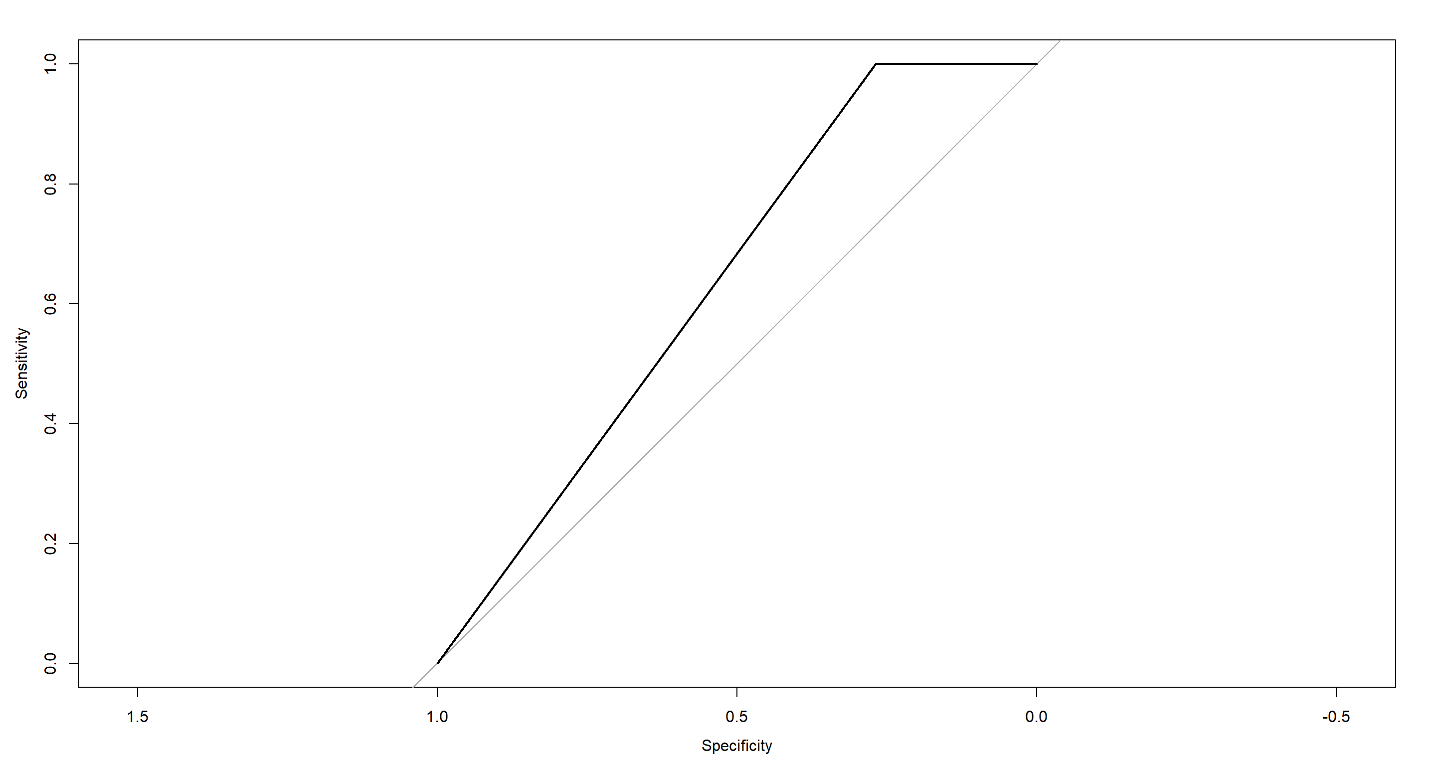
auc(Mclust_PS.roc)
## Area under the curve: 0.6341
Certainly, we could do better! Let’s see what more advanced methods have to offer.
With that, we turn to random forest:
RF_PS.roc <- roc(
  Sparrows_df$Population.Status,
  H2_PS_RF$votes[, 1]
)
plot(RF_PS.roc)
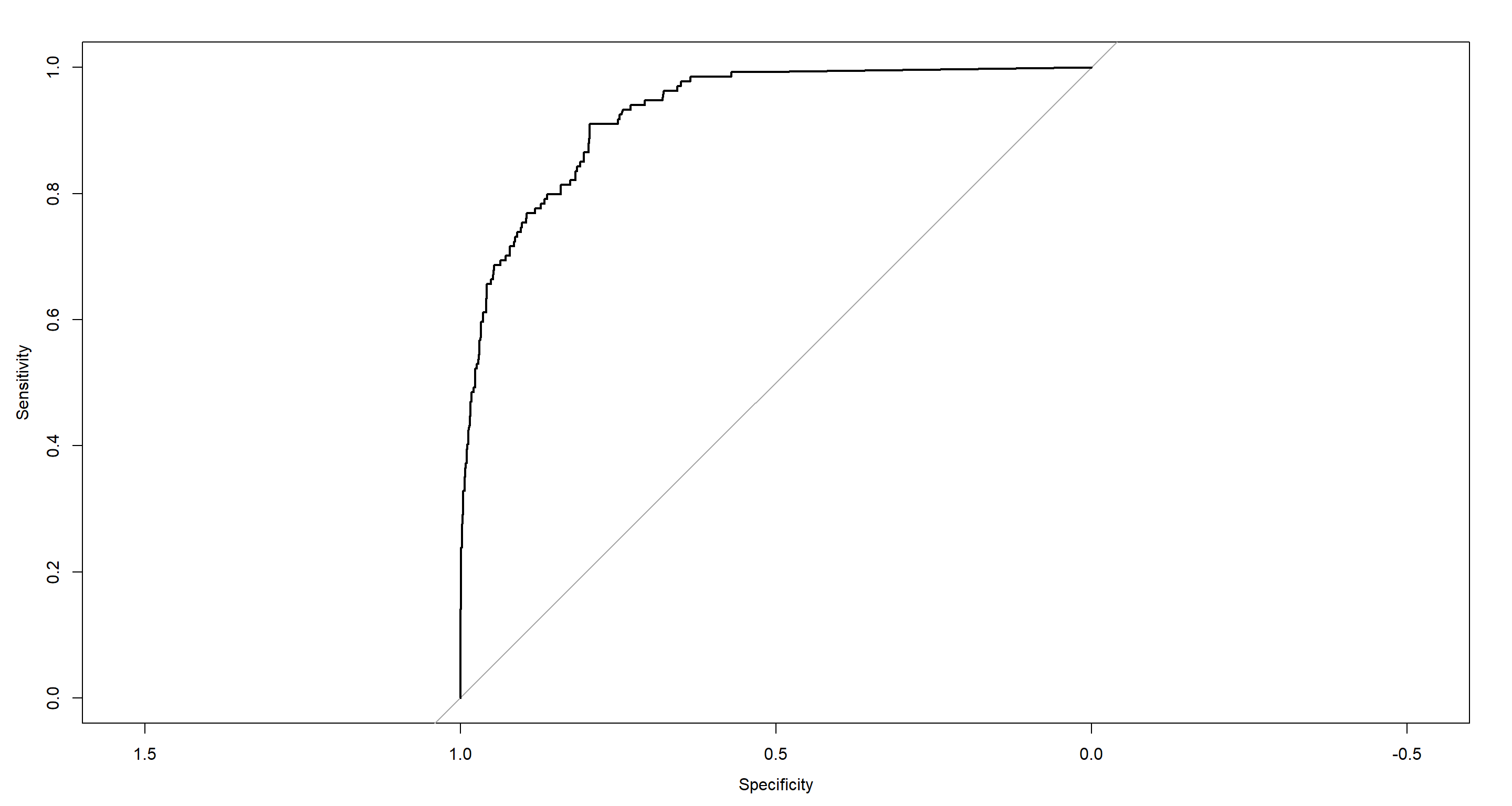
auc(RF_PS.roc)
## Area under the curve: 0.9274
Now this is doing much better!
Lastly, we want to look at the site Index as predicted by sparrow morphology given a random forest algorithm:
RF_Index.roc <- multiclass.roc(
  Sparrows_df$Index, # known outcome
  H2_Index_RF$votes # matrix of certainties of prediction
)
RF_Index.roc[["auc"]] # average ROC-AUC
## Multi-class area under the curve: 0.9606
## Plot ROC curve for each binary comparison
rs <- RF_Index.roc[["rocs"]] ## extract comparisons
plot.roc(rs[[1]][[1]]) # blot first comparison
plot.roc(rs[[1]][[2]], add = TRUE) # plot first comparison, in opposite direction
invisible(capture.output(sapply(2:length(rs), function(i) lines.roc(rs[[i]][[1]], col = i))))
invisible(capture.output(sapply(2:length(rs), function(i) lines.roc(rs[[i]][[2]], col = i))))
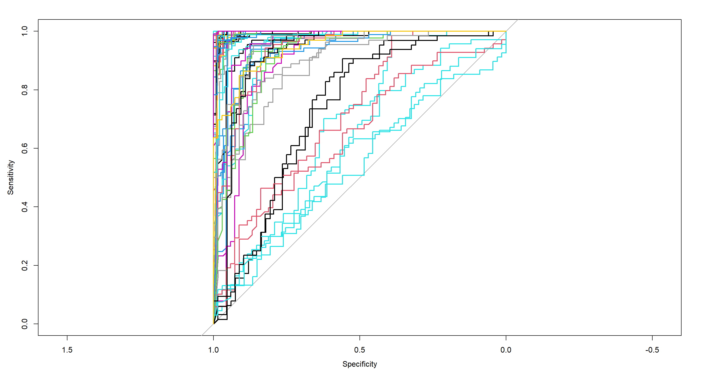
This is certainly busy, but look at that average AUC of almost 1! That is the power of Random Forest.
Summary of Model Selection
Morphology Hypothesis
Regarding our morphology hypothesis, we saw that most of our hypothesised effects can be detected. However, some models clearly perform better than others. Usual model selection exercises would have us discard all but the best model (Full, in this case) and leave the rest never to be spoken of again. Doing so would have us miss a pretty neat opportunity to do some model comparison which can already help us identify which effects to focus on in particular.
To demonstrate some of this, allow me step into the local regression models:
sapply(H1_ModelCNA_ls, AIC)
##       Null  Clim_TAvg   Clim_TSD  Clim_Full  Pred_Pres  Pred_Type       Full Mixed_Full
##   948.7346   882.9998   851.9833   846.2997   941.2811   846.2997   844.6250   875.7659
as well as global regression models:
sapply(H1_Model_ls, AIC)
##            Null Comp_Flock.Size       Comp_Full            Full      Mixed_Full
##        6019.872        4389.378        4286.445        4047.250        4162.779
- Climate - interestingly, temperature variability is much more informative than average temperature and even adding the two into the same model only marginally improves over the variability-only model. This tells us much about which effects are probably meaningful and which aren’t.
- Competition - The competition models did well across the board, but were aided immensely by adding climate information and accounting for random effects.
- Predation - predation effects were best explained by predation type with only a marginal improvement of adding predator presence. That is because predator type already contains all of the information that is within predator presence.
What we can do so far, is remove some obviously erroneous models which in this case is the entirety of local regression models.
Categorisation Hypothesis
As far as the categorisation hypotheses are concerned, we now have confirmation that population status and sparrow morphology are linked quite well.
We have also learned that random forest is an incredibly powerful method for classification and variable selection.
Model Validation
So far, we have not introduced our models to any new data. We have looked at explanatory power with (adjusted) $R^2$, and the Anova. We have also looked at estimates of predictive power with our information criteria (e.g. AIC, BIC).
What about actually seeing how robust and accurate our models are? That’s what Model Validation is for!
Cross-Validation
Before we get started, I remove the Null model from our model list. Doing cross-validation on this does not make any sense because there are no actual predictors in it which could be affected by cross-validation processes.
H1_Model_ls <- H1_Model_ls[-1]
Training vs. Test Data
The simplest example of cross-validation is the validation data cross-validation approach; also known as Training vs. Test Data approach.
To make use of this approach, we need to (1) randomly split our data, (2) build our models using the training data, and (3) test our models on the test data.
Since we have highly compartmentalised data at different sites, I am employing a stratified sampling scheme to ensure all of my sites are represented in each data set resulting from the split:
set.seed(42) # make randomness reproducible
Stratified_ls <- stratified(Sparrows_df, # what to split
  group = "Index", # by which group to stratify
  size = .7, # what proportion of each group shall be contained in the training data
  bothSets = TRUE # save both training and test data
)
Train_df <- Stratified_ls$SAMP1 # extract training data
Test_df <- Stratified_ls$SAMP2 # extract test data
Now that we have our training and test data, we are ready to run our pre-specified models on said data and subsequently test it’s performance on the test data by predicting with the newly trained model and calculating mean squared test error.
For a single model, we can do it like this:
ExampleModel <- H1_ModelSparrows_ls$Comp_Flock.Size # extract Model from list
ExampleModel <- update(ExampleModel, data = Train_df) # train model on training data
Prediction <- predict(ExampleModel, newdata = Test_df) # predict outcome for test data
sum((Test_df$Weight - Prediction)^2) # Mean Squared Error
## [1] 1133.996
Since we have multiple models stored in a list, here’s a way to do the above for the entire list:
H1_Train_ls <- sapply(X = H1_Model_ls, FUN = function(x) update(x, data = Train_df))
H1_Test_mat <- sapply(X = H1_Train_ls, FUN = function(x) predict(x, newdata = Test_df))
apply(H1_Test_mat, MARGIN = 2, FUN = function(x) sum((Test_df$Weight - x)^2))
## Comp_Flock.Size       Comp_Full            Full      Mixed_Full
##       1133.9958       1026.2199        816.5166        866.2941
Again, our full model comes out on top!
Unfortunately, this approach is fickle due to the randomness of the data split. How can we make this more robust? Easy. We split many, many times and average our mean squared errors out.
This bring us to traditional Cross-Validation approaches. Luckily, the complex parts of cross-validation are already offered to us with the caret package in R
Leave-One-Out Cross-Validation (LOOCV)
Leave-One-Out Cross-Validation is a method within which we split our data into a training data set with $n-1$ observation and a test data set that contains just $1$ observation. We do training and testing as above on this split and then repeat this procedure until every observation has been left out once.
For a simple model, this can be done like such:
train(Weight ~ Climate,
  data = Sparrows_df,
  method = "lm",
  trControl = trainControl(method = "LOOCV")
)
## Linear Regression
##
## 1066 samples
##    1 predictor
##
## No pre-processing
## Resampling: Leave-One-Out Cross-Validation
## Summary of sample sizes: 1065, 1065, 1065, 1065, 1065, 1065, ...
## Resampling results:
##
##   RMSE      Rsquared   MAE
##   3.628905  0.2036173  2.976221
##
## Tuning parameter 'intercept' was held constant at a value of TRUE
Notice the RMSE (Residual mean squared error). That’s what we use to compare models.
Here, I create a function that automatically rebuilds our models for the LOOCV so we can run this on our list of models later.
CV_LOOCV <- function(x) {
  if (length(x[["terms"]][[3]]) == 1) {
    Terms <- paste(x[["terms"]][[3]], collapse = " + ")
  } else {
    Terms <- paste(x[["terms"]][[3]][-1], collapse = " + ")
  }
  train(as.formula(paste("Weight ~", Terms)),
    data = Sparrows_df,
    method = "lm",
    trControl = trainControl(method = "LOOCV")
  )
}
Unfortunately, this cannot be executed for mixed effect models, so for now, I only run this on all our models except the mixed effect model:
Begin <- Sys.time()
H1_LOOCV_ls <- sapply(H1_Model_ls[-length(H1_Model_ls)], CV_LOOCV)
End <- Sys.time()
End - Begin
## Time difference of 9.41841 secs
sapply(H1_LOOCV_ls, "[[", "results")[-1, ]
##          Comp_Flock.Size Comp_Full Full
## RMSE     1.894279        1.865854  1.609296
## Rsquared 0.7829992       0.7894634 0.8433834
## MAE      1.520181        1.492409  1.279003
Unsurprisingly, our full model has the lowest RMSE (which is the mark of a good model).
So what about our mixed effect model? Luckily, doing LOOCV by hand isn’t all that difficult and so we can still compute a RMSE for LOOCV for our mixed effect model:
RMSE_LOOCV <- rep(NA, nrow(Sparrows_df))
for (Fold_Iter in 1:nrow(Sparrows_df)) {
  Iter_mod <- update(H1_Model_ls$Mixed_Full, data = Sparrows_df[-Fold_Iter, ])
  Prediction <- predict(Iter_mod, newdata = Sparrows_df[Fold_Iter, ])
  RMSE_LOOCV[Fold_Iter] <- (Sparrows_df[Fold_Iter, ]$Weight - Prediction)^2
}
mean(RMSE_LOOCV)
## [1] 2.757373
Ouh… that is quite worse than out other models. Curious. This goes to show how much less robust a more complex model can be.
k-Fold Cross-Validation (k-fold CV)
k-Fold Cross-Validation uses the same concept as all of the previous cross-validation methods, but at less of a computational cost than LOOCV and more robustly than the training/test data approach:
Again, I write a function for this and run it on my list of models without the mixed effect model:
CV_kFold <- function(x) {
  if (length(x[["terms"]][[3]]) == 1) {
    Terms <- paste(x[["terms"]][[3]], collapse = " + ")
  } else {
    Terms <- paste(x[["terms"]][[3]][-1], collapse = " + ")
  }
  train(as.formula(paste("Weight ~", Terms)),
    data = Sparrows_df,
    method = "lm",
    trControl = trainControl(method = "cv", number = 15)
  )
}
Begin <- Sys.time()
H1_kFold_ls <- sapply(H1_Model_ls[-length(H1_Model_ls)], CV_kFold)
End <- Sys.time()
End - Begin
## Time difference of 0.3413441 secs
sapply(H1_kFold_ls, "[[", "results")[-1, ]
##            Comp_Flock.Size Comp_Full  Full
## RMSE       1.889439        1.859135   1.603168
## Rsquared   0.7882333       0.7942782  0.8465977
## MAE        1.519962        1.491493   1.277595
## RMSESD     0.1408563       0.1520344  0.1491081
## RsquaredSD 0.03375562      0.03153792 0.03034729
## MAESD      0.1382304       0.1122565  0.1150599
Full model performs best still and see how much quicker that was done!
Bootstrap
On to the Bootstrap. God, I love the boostrap.
The idea here is to run a model multiple times on a random sample of the underlying data and then store all of the estimates or the parameters as well as avaerage out the RMSE:
BootStrap <- function(x) {
  if (length(x[["terms"]][[3]]) == 1) {
    Terms <- paste(x[["terms"]][[3]], collapse = " + ")
  } else {
    Terms <- paste(x[["terms"]][[3]][-1], collapse = " + ")
  }
  train(as.formula(paste("Weight ~", Terms)),
    data = Sparrows_df,
    method = "lm",
    trControl = trainControl(method = "boot", number = 100)
  )
}
Begin <- Sys.time()
H1_BootStrap_ls <- sapply(H1_Model_ls[-length(H1_Model_ls)], BootStrap)
End <- Sys.time()
End - Begin
## Time difference of 1.308739 secs
sapply(H1_BootStrap_ls, "[[", "results")[-1, ]
##            Comp_Flock.Size Comp_Full  Full
## RMSE       1.893652        1.871873   1.622079
## Rsquared   0.7835412       0.7896534  0.8425108
## MAE        1.520457        1.498216   1.288087
## RMSESD     0.04675792      0.05178669 0.04885059
## RsquaredSD 0.01243994      0.01318599 0.01092356
## MAESD      0.04287091      0.04531032 0.03910463
The full model is still doing great, of course.
But what about our mixed effect model? Luckily, there is a function that can do bootstrapping for us on our lme objects:
## Bootstrap mixed model
Mixed_boot <- lmeresampler::bootstrap(H1_Model_ls[[length(H1_Model_ls)]], .f = fixef, type = "parametric", B = 3e3)
Mixed_boot
## Bootstrap type: parametric
##
## Number of resamples: 3000
##
##                           term      observed      rep.mean          se          bias
## 1                  (Intercept)  2.212717e+01 22.0672111291 2.853845096 -0.0599612233
## 2       Predator.TypeNon-Avian  6.626664e-01  0.6580310750 0.161081567 -0.0046353000
## 3            Predator.TypeNone  2.694373e-02  0.0212966961 0.152739708 -0.0056470340
## 4                   Flock.Size  1.497092e-05  0.0005839265 0.019216411  0.0005689556
## 5             Home.RangeMedium  1.261878e+00  1.2675791500 0.881426872  0.0057008365
## 6              Home.RangeSmall  3.049068e+00  3.0583903125 0.417796779  0.0093225898
## 7                         TAvg  3.015153e-02  0.0303345903 0.009892483  0.0001830556
## 8                          TSD  1.983744e-01  0.1984962823 0.021196164  0.0001219321
## 9  Flock.Size:Home.RangeMedium -1.208598e-01 -0.1213017777 0.057929474 -0.0004419594
## 10  Flock.Size:Home.RangeSmall -2.110972e-01 -0.2117971129 0.019731749 -0.0006998822
##
## There were 0 messages, 0 warnings, and 0 errors.
With this, we are getting into the heart of the bootstrap. Distributions of our parameter estimates. These give us an amazing understanding of just which parameter values our model sees as plausible given our data:
Estimates_df <- data.frame(Mixed_boot[["replicates"]])
## reshape estimates data frame for plotting
Hist_df <- data.frame(pivot_longer(
  data = Estimates_df,
  cols = colnames(Estimates_df)
))
## plot parameter estimate distributions
ggplot(data = Hist_df, aes(x = value, group = name)) +
  tidybayes::stat_pointinterval() +
  tidybayes::stat_dots() +
  facet_wrap(~name, scales = "free") +
  labs(
    x = "Parameter Estimate", y = "Parameter",
    title = paste("Bootstrap parameter estimates of", names(H1_Model_ls[[length(H1_Model_ls)]]), "Model")
  ) +
  theme_bw()
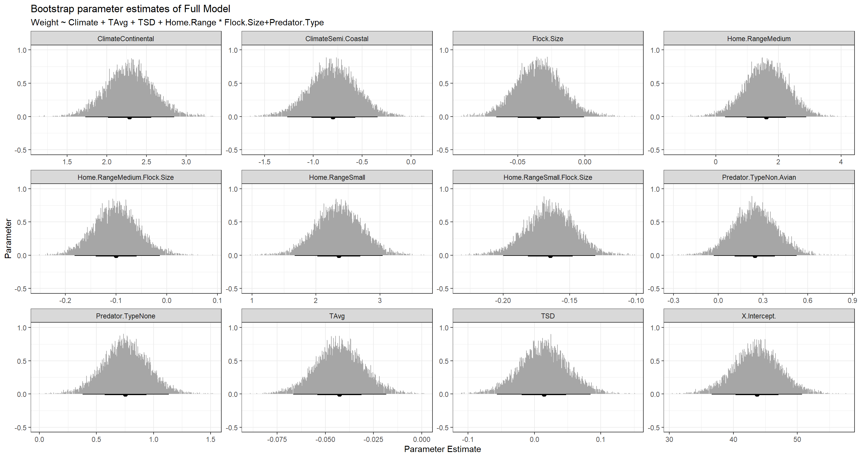
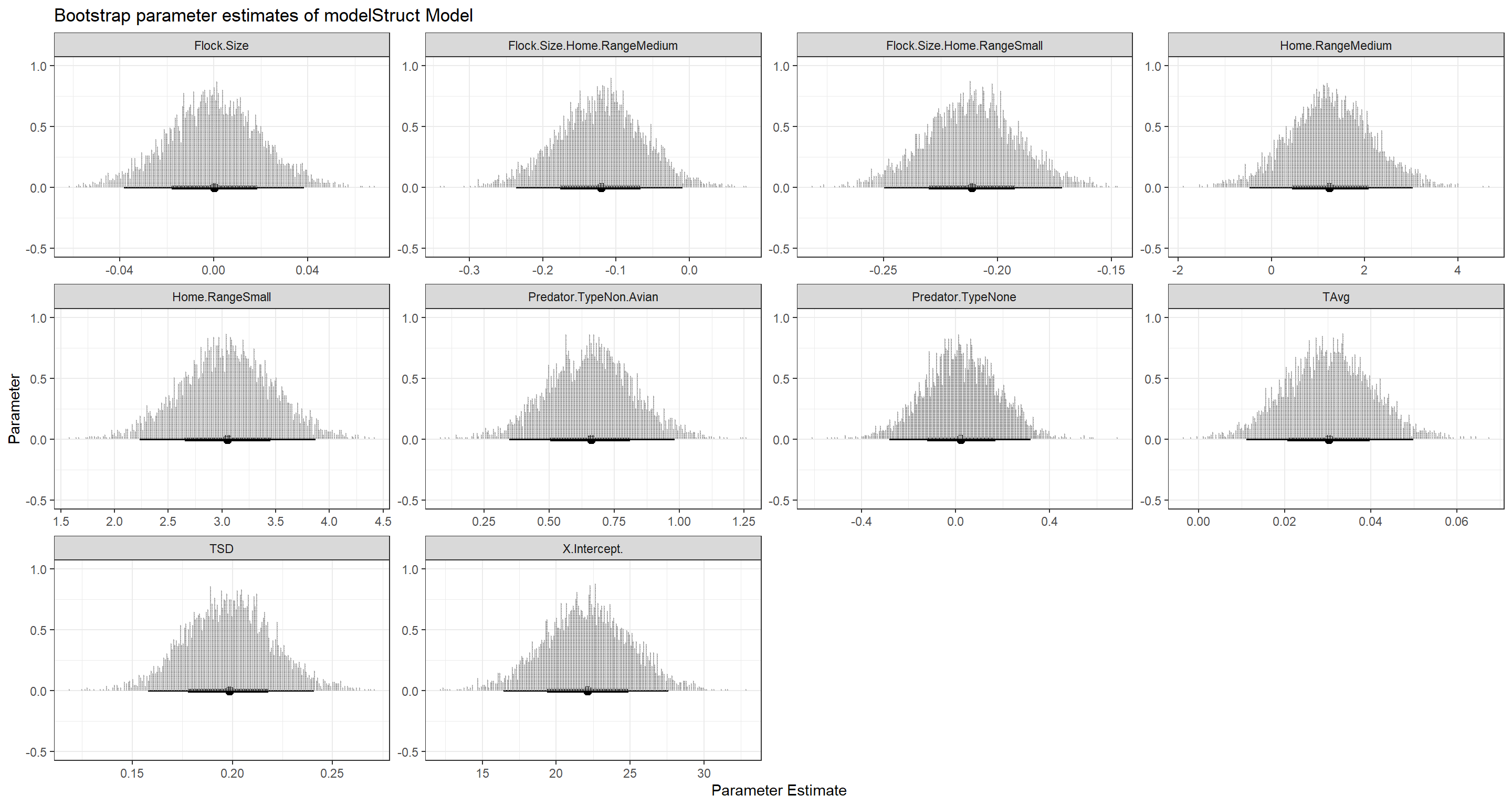 As you can see for our mixed effect model, while most parameter estimates are nicely constrained, the Intercept estimate can vary wildly. This is likely to do with our model being very flexible and allowing for a bunch of different combinations of intercepts.
Let’s do the same for our remaining three candidate models:
BootPlot_ls <- as.list(rep(NA, (length(H1_Model_ls) - 1)))
for (Model_Iter in 1:(length(H1_Model_ls) - 1)) { # loop over all models except the null model
  ## Formula to compute coefficients
  x <- H1_Model_ls[[Model_Iter]]
  if (length(x[["terms"]][[3]]) == 1) {
    Terms <- as.character(x[["terms"]][[3]])
  } else {
    Terms <- paste(as.character(x[["terms"]][[3]])[-1], collapse = as.character(x[["terms"]][[3]])[1])
  }
  model_coef <- function(data, index) {
    coef(lm(as.formula(paste("Weight ~", Terms)), data = data, subset = index))
  }
  ## Bootstrapping
  Boot_test <- boot(data = Sparrows_df, statistic = model_coef, R = 3e3)
  ## set column names of estimates to coefficients
  colnames(Boot_test[["t"]]) <- names(H1_Model_ls[[Model_Iter]][["coefficients"]])
  ## make data frame of estimates
  Estimates_df <- data.frame(Boot_test[["t"]])
  ## reshape estimates data frame for plotting
  Hist_df <- data.frame(pivot_longer(
    data = Estimates_df,
    cols = colnames(Estimates_df)
  ))
  ## plot parameter estimate distributions
  BootPlot_ls[[Model_Iter]] <- ggplot(data = Hist_df, aes(x = value, group = name)) +
    tidybayes::stat_pointinterval() +
    tidybayes::stat_dots() +
    facet_wrap(~name, scales = "free") +
    labs(
      x = "Parameter Estimate", y = "Parameter",
      title = paste("Bootstrap parameter estimates of", names(H1_Model_ls)[[Model_Iter]], "Model"),
      subtitle = paste("Weight ~", Terms)
    ) +
    theme_bw()
}
BootPlot_ls[[1]]
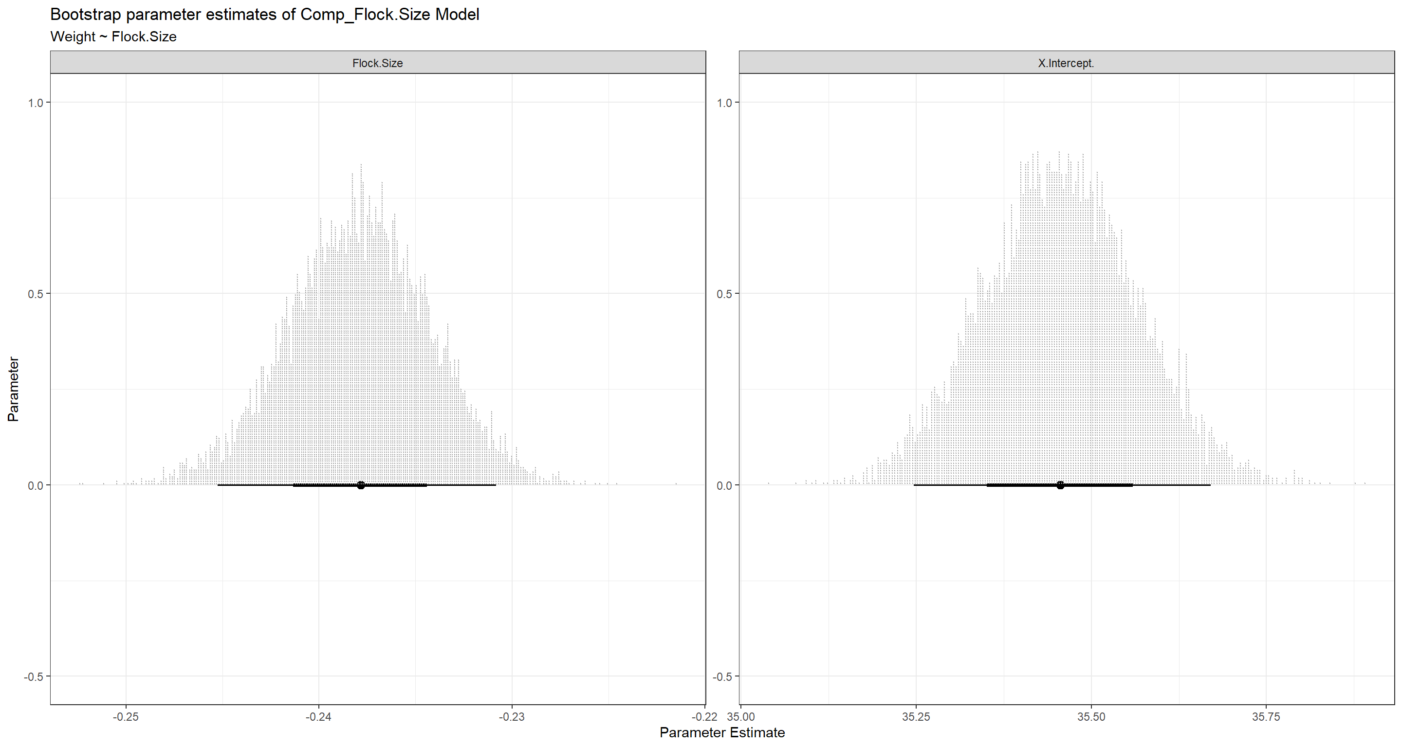
BootPlot_ls[[2]]
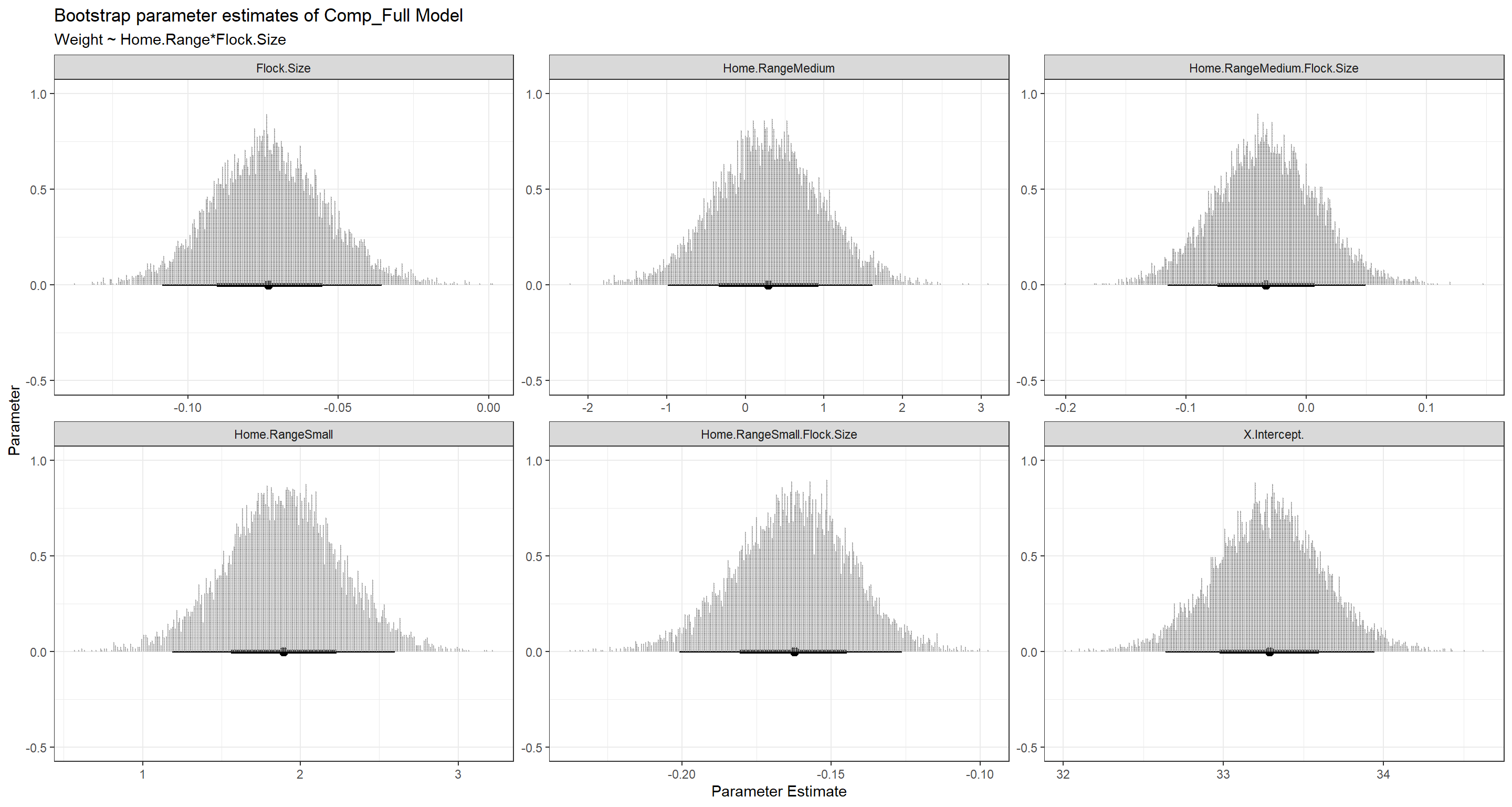
BootPlot_ls[[3]]
Subset Selection
So far, we have built our own models according to out intuition. Did we test all possible models? No. Should we go back and test all possible models by hand? Hell no! Can we let R do it for us? You bet we can!
Best Subset Selection
Let’s start with best subset selection. Doing so asks us/R to establish all possible models and then select the one that performs best according to information criteria. Because our data set contains over 20 variables, including all of our variables would have us establish close to 1 million (you read that right) models. THat is, of course, infeasible.
Therefore, let’s just allow our subset selection to use all variables we have used ourselves thus far (with the exclusion of Index because it’s an amazing, but ultimately useless shorthand):
Reduced_df <- Sparrows_df[, c("Weight", "Climate", "TAvg", "TSD", "Population.Status", "Flock.Size", "Predator.Type", "Predator.Presence")] # reduce data
model <- lm(Weight ~ ., data = Reduced_df) # specify full model
k <- ols_step_best_subset(model) # create all models and select the best
k # show us comparison of best subsets
##                                   Best Subsets Regression
## --------------------------------------------------------------------------------------------
## Model Index    Predictors
## --------------------------------------------------------------------------------------------
##      1         Flock.Size
##      2         Climate Flock.Size
##      3         Climate TAvg Flock.Size
##      4         Climate TAvg Flock.Size Predator.Type
##      5         Climate TAvg TSD Flock.Size Predator.Type
##      6         Climate TAvg TSD Population.Status Flock.Size Predator.Type
##      7         Climate TAvg TSD Population.Status Flock.Size Predator.Type Predator.Presence
## --------------------------------------------------------------------------------------------
##
##                                                     Subsets Regression Summary
## ----------------------------------------------------------------------------------------------------------------------------------
##                        Adj.        Pred
## Model    R-Square    R-Square    R-Square      C(p)         AIC       SBIC       SBC         MSEP        FPE       HSP       APC
## ----------------------------------------------------------------------------------------------------------------------------------
##   1        0.7838      0.7836       0.783    298.7733    4389.3782      NA    4404.2932    3818.6664    3.5890    0.0034    0.2170
##   2        0.8175      0.8169      0.8163     88.8025    4212.8692      NA    4237.7276    3226.8597    3.0384    0.0029    0.1836
##   3        0.8227      0.8220      0.8213     58.0852    4184.0693      NA    4213.8994    3137.9149    2.9575    0.0028    0.1787
##   4        0.8315      0.8305      0.8296      4.5702    4133.6815      NA    4173.4549    2984.6456    2.8183    0.0026    0.1701
##   5        0.8320      0.8309      0.8298      3.3977    4132.4880      NA    4177.2330    2978.5274    2.8151    0.0026    0.1699
##   6        0.8320      0.8308      0.8296      5.0000    4134.0870      NA    4183.8036    2980.2214    2.8194    0.0026    0.1702
##   7        0.8320      0.8308      0.8296      5.0000    4136.0870      NA    4190.7753    2980.2214    2.8194    0.0026    0.1702
## ----------------------------------------------------------------------------------------------------------------------------------
## AIC: Akaike Information Criteria
##  SBIC: Sawa's Bayesian Information Criteria
##  SBC: Schwarz Bayesian Criteria
##  MSEP: Estimated error of prediction, assuming multivariate normality
##  FPE: Final Prediction Error
##  HSP: Hocking's Sp
##  APC: Amemiya Prediction Criteria
Model 5 (Climate TAvg TSD Flock.Size Predator.Type ) is the one we want to go for here.
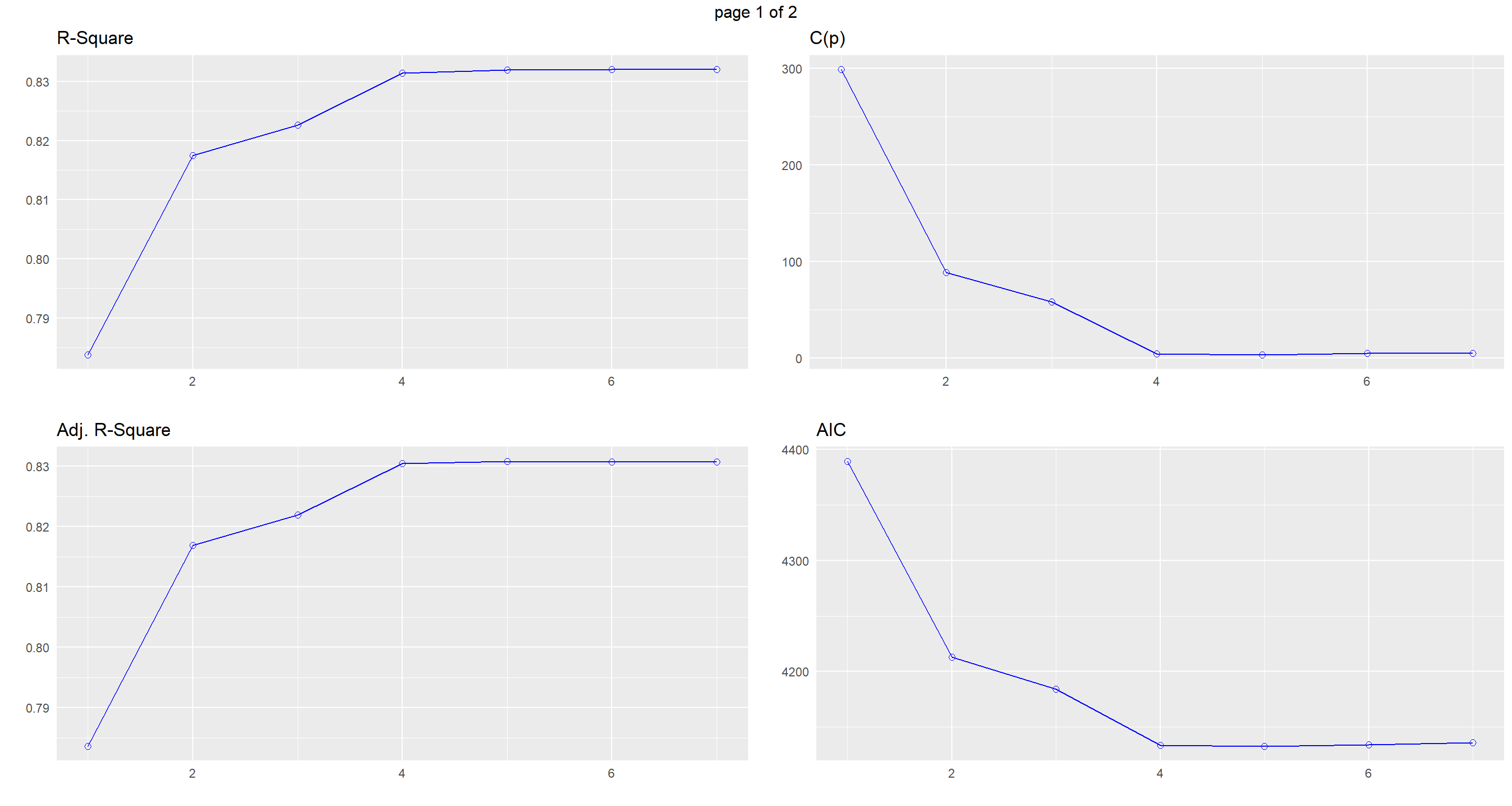
Let’s look at visualisation of our different model selection criteria:
plot(k)
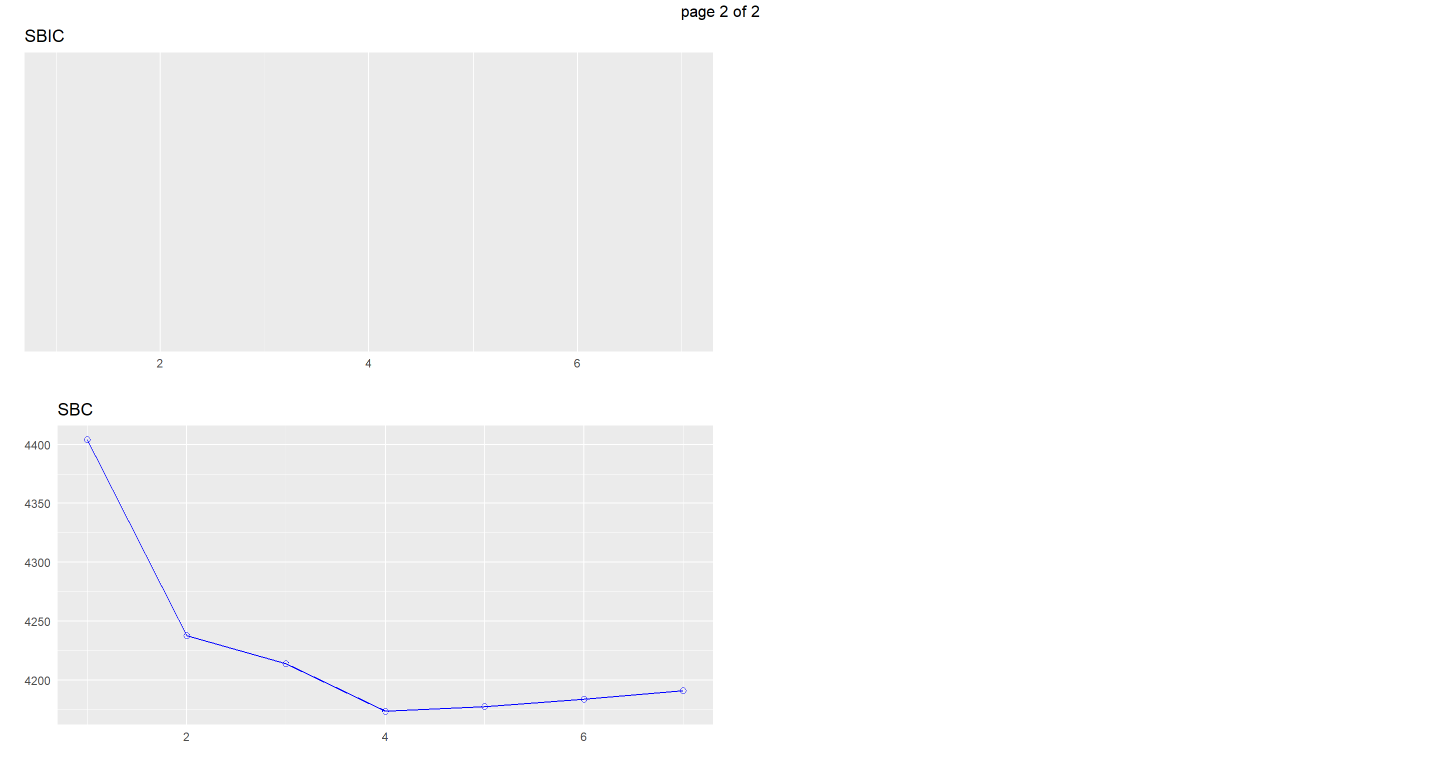
Forward Subset Selection
Ok. So best subset selection can become intractable given a lot of variables. How about building our models up to be increasingly complex until we hit on gold?
Unfortunately, doing so does not guarantee finding an optimal model and can easily get stuck, depending on what the model starts off with:
model <- lm(Weight ~ Climate, data = Reduced_df)
step.model <- stepAIC(model,
  direction = "forward",
  trace = FALSE
)
summary(step.model)
##
## Call:
## lm(formula = Weight ~ Climate, data = Reduced_df)
##
## Residuals:
##    Min     1Q Median     3Q    Max
## -9.020 -2.033  1.050  2.640  6.610
##
## Coefficients:
##                     Estimate Std. Error t value Pr(>|t|)
## (Intercept)          28.3998     0.1248 227.628  < 2e-16 ***
## ClimateContinental    4.9785     0.3188  15.616  < 2e-16 ***
## ClimateSemi-Coastal   3.3400     0.4606   7.252  7.9e-13 ***
## ---
## Signif. codes:  0 '***' 0.001 '**' 0.01 '*' 0.05 '.' 0.1 ' ' 1
##
## Residual standard error: 3.629 on 1063 degrees of freedom
## Multiple R-squared:  0.2059,	Adjusted R-squared:  0.2044
## F-statistic: 137.8 on 2 and 1063 DF,  p-value: < 2.2e-16
We immediately remain on Climate as the only predictor in this example.
What if we start with a true null model?
model <- lm(Weight ~ 1, data = Reduced_df)
step.model <- stepAIC(model,
  direction = "forward",
  trace = FALSE
)
summary(step.model)
##
## Call:
## lm(formula = Weight ~ 1, data = Reduced_df)
##
## Residuals:
##    Min     1Q Median     3Q    Max
## -9.944 -1.452  1.291  2.913  7.336
##
## Coefficients:
##             Estimate Std. Error t value Pr(>|t|)
## (Intercept)  29.3243     0.1246   235.3   <2e-16 ***
## ---
## Signif. codes:  0 '***' 0.001 '**' 0.01 '*' 0.05 '.' 0.1 ' ' 1
##
## Residual standard error: 4.068 on 1065 degrees of freedom
We even get stuck on our null model!
Backward Subset Selection
So what about making our full model simpler?
model <- lm(Weight ~ ., data = Reduced_df)
step.model <- stepAIC(model,
  direction = "backward",
  trace = FALSE
)
summary(step.model)
##
## Call:
## lm(formula = Weight ~ Climate + TAvg + TSD + Flock.Size + Predator.Type,
##     data = Reduced_df)
##
## Residuals:
##     Min      1Q  Median      3Q     Max
## -5.2398 -1.1180  0.1215  1.1474  4.9151
##
## Coefficients:
##                         Estimate Std. Error t value Pr(>|t|)
## (Intercept)            53.505428   3.748484  14.274  < 2e-16 ***
## ClimateContinental      2.978894   0.301131   9.892  < 2e-16 ***
## ClimateSemi-Coastal    -0.640161   0.310970  -2.059   0.0398 *
## TAvg                   -0.068582   0.012713  -5.395 8.47e-08 ***
## TSD                    -0.069306   0.038900  -1.782   0.0751 .
## Flock.Size             -0.189607   0.005122 -37.019  < 2e-16 ***
## Predator.TypeNon-Avian  0.379606   0.161332   2.353   0.0188 *
## Predator.TypeNone       1.258391   0.165347   7.611 6.02e-14 ***
## ---
## Signif. codes:  0 '***' 0.001 '**' 0.01 '*' 0.05 '.' 0.1 ' ' 1
##
## Residual standard error: 1.673 on 1058 degrees of freedom
## Multiple R-squared:  0.832,	Adjusted R-squared:  0.8309
## F-statistic: 748.4 on 7 and 1058 DF,  p-value: < 2.2e-16
Interesting. This time, we have hit on the same model that was identified by the best subset selection above.
Forward & Backward
Can we combine the directions of stepwise model selection? Yes, we can:
model <- lm(Weight ~ ., data = Reduced_df)
step.model <- stepAIC(model,
  direction = "both",
  trace = FALSE
)
summary(step.model)
##
## Call:
## lm(formula = Weight ~ Climate + TAvg + TSD + Flock.Size + Predator.Type,
##     data = Reduced_df)
##
## Residuals:
##     Min      1Q  Median      3Q     Max
## -5.2398 -1.1180  0.1215  1.1474  4.9151
##
## Coefficients:
##                         Estimate Std. Error t value Pr(>|t|)
## (Intercept)            53.505428   3.748484  14.274  < 2e-16 ***
## ClimateContinental      2.978894   0.301131   9.892  < 2e-16 ***
## ClimateSemi-Coastal    -0.640161   0.310970  -2.059   0.0398 *
## TAvg                   -0.068582   0.012713  -5.395 8.47e-08 ***
## TSD                    -0.069306   0.038900  -1.782   0.0751 .
## Flock.Size             -0.189607   0.005122 -37.019  < 2e-16 ***
## Predator.TypeNon-Avian  0.379606   0.161332   2.353   0.0188 *
## Predator.TypeNone       1.258391   0.165347   7.611 6.02e-14 ***
## ---
## Signif. codes:  0 '***' 0.001 '**' 0.01 '*' 0.05 '.' 0.1 ' ' 1
##
## Residual standard error: 1.673 on 1058 degrees of freedom
## Multiple R-squared:  0.832,	Adjusted R-squared:  0.8309
## F-statistic: 748.4 on 7 and 1058 DF,  p-value: < 2.2e-16
Again, we land on our best subset selection model!
Subset Selection vs. Our Intuition
Given our best subset selection, we have a very good idea of which model to go for.
To see how well said model shapes up against our full model, we can simply look at LOOCV:
train(Weight ~ Climate + TAvg + TSD + Flock.Size + Predator.Type,
  data = Sparrows_df,
  method = "lm",
  trControl = trainControl(method = "LOOCV")
)
## Linear Regression
##
## 1066 samples
##    5 predictor
##
## No pre-processing
## Resampling: Leave-One-Out Cross-Validation
## Summary of sample sizes: 1065, 1065, 1065, 1065, 1065, 1065, ...
## Resampling results:
##
##   RMSE      Rsquared   MAE
##   1.677673  0.8297908  1.338399
##
## Tuning parameter 'intercept' was held constant at a value of TRUE
sapply(H1_LOOCV_ls, "[[", "results")[-1, ]
##          Comp_Flock.Size Comp_Full Full
## RMSE     1.894279        1.865854  1.609296
## Rsquared 0.7829992       0.7894634 0.8433834
## MAE      1.520181        1.492409  1.279003
And our full model still wins! But why? Didn’t we test for all models? Yes, we tested for all additive models, but our Full model contains an interaction terms which the automated functions above just cannot handle, sadly.
Let’s ask a completely different question. Would we have even adopted the best subset selection model if we had thought of it given the assumptions of a linear regression?
par(mfrow = c(2, 2))
plot(lm(Weight ~ Climate + TAvg + TSD + Flock.Size + Predator.Type, data = Sparrows_df))
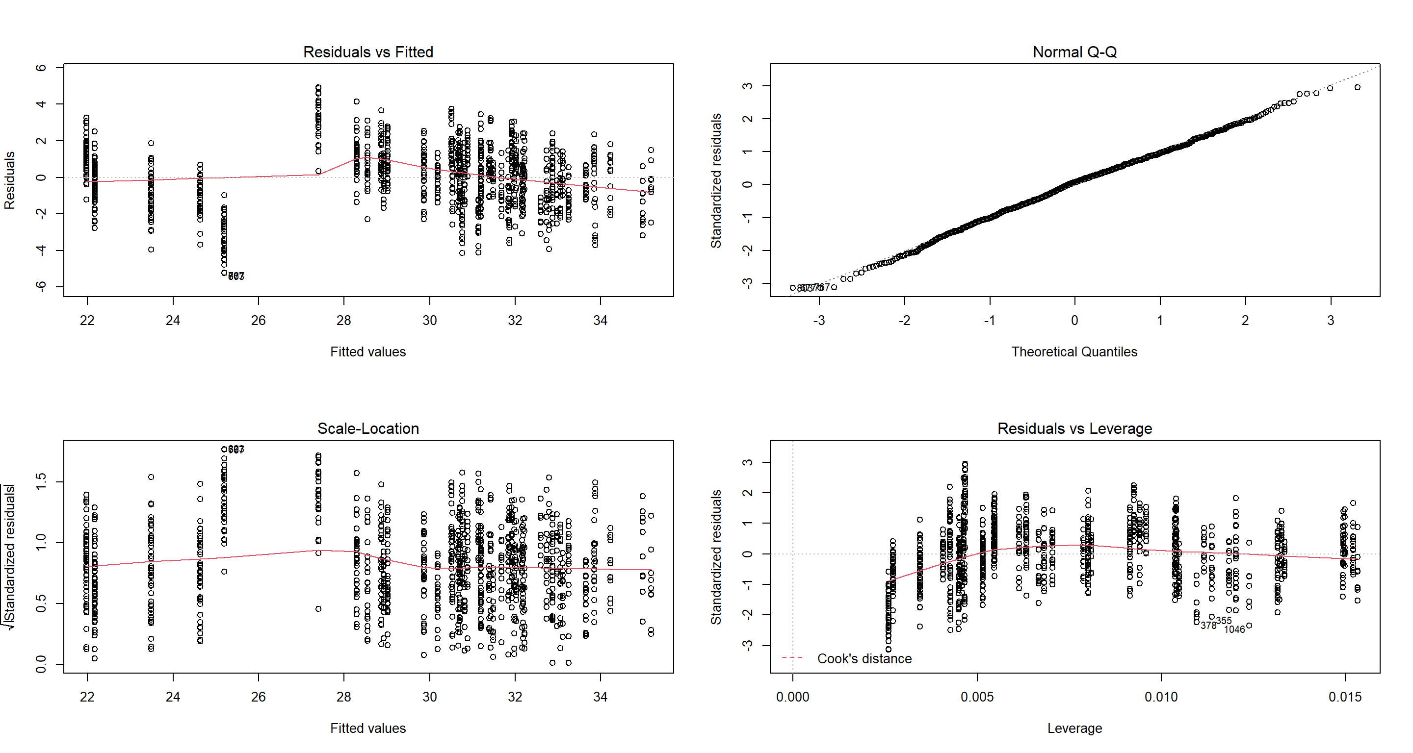
As it turns out, this is a perfectly reasonable model. It’s just not as good as our full model.